We’ve all heard the rather derogatory phrase “Lies, Damn Lies, and Statistics”. Apparently it’s origin is attributed to British prime minister Benjamin Disraeli, via Mark Twain, at the turn of the 19th century. While this apocryphal phrase could possibly reflect some of the more dubious studies in the socio-political sciences that are (too often?) published today, this is certainly not the case when it comes to the serious physical sciences. Here, statistical analyses of experimental data and measurements have proven time and time again to be extremely useful.
So in this article I am going to outline how statistical methods can be applied to spectroscopy. If you are already beginning to yawn and are losing interest at the mere mention of the word statistics, I ask for your indulgence for the short time it will take you to read this article. And then again, there are many other topics for you to explore elsewhere at Steve’s Open Lab.
So let’s begin if you are not too statistics averse 😊
Chemometrics
The discipline of chemometrics is relatively new as sciences go. Its modern origins can be traced back to the application of computers in chemical research labs in the early 1970’s. Not surprisingly, this parallels the development and introduction of minicomputers and PC’s, when researchers began to apply mathematical and statistical methods to solving chemical problems.
Wikipedia defines chemometrics as “the science of extracting information from chemical systems by data-driven means”. That’s a bit too general in my personal opinion, but chemometrics is multidisciplinary in nature. There are better definitions and many have been proposed. In essence, chemometrics applies well established mathematical and statistical methods such a regression, ANOVA, Partial Least Squares (PLS) Principle Components Analysis and associated techniques to solve complex problems in the chemical sciences.
Although nascent developments in the techniques understandably arose in the research lab, especially on the software and computational side of things, the rapid developments in chemometrics have today reached a high degree of sophistication. They have achieved recognition and acceptance by scientists and engineers. This has led to chemometric methods being developed and refined that are capable of monitoring chemical manufacturing processes in pseudo-real time to monitor any variability in product quality.
So let’s now consider a practical example of the use of chemometrics in a spectroscopic problem. Just for fun, I am going to do this by way of a story! Although fictional, this story is typical in many ways of a real-life investigative problem in an industrial environment.
Here we go…
A Chemometrics Story
Setting the Scene
You are a research chemist working in the R&D department of a large chemical company. The company manufactures a range of organic compounds, and one of the company’s flagship products is a high purity grade of methanol, CH3OH.
In recent days the QC (Quality Control) department has noticed a random and intermittent contamination in the methanol production line by the presence of acetone. Process engineers in the manufacturing plant are working overtime trying to trace the source of the contamination, but their search continues.
Contaminated methanol batches have had to be rejected by QC. Rejected batches means production loss, revenue loss and directly affects the company’s bottom line. Senior management needs to know what is going on, whether the problem will continue and “a solution needs to be found fast!” The QC department has passed on the issue to the R&D department and the problem has arrived on your desk 😒
You know that the QC department will require an SOP (Standard Operating Procedure) capable of predicting the purity of future batches of methanol with a clear procedure on how to determine and measure any trends in batch quality. This will then enable the department to set up working specifications and quality control limits for this important company product.
Approaching the Problem
A few months ago the R&D department purchased an interesting and useful chemometrics software package called PEAXACT. You have been trained up in its use and are quite familiar with this app. You recognise that this is a good opportunity to use the software in analysing the acetone contamination issue.
PEAXACT software is an interactive app for the quantitative analysis of spectra obtained from the typical spectroscopic instruments found in chemistry labs: UV-Visible, FTIR and Raman spectrometers. The app employs chemometric techniques to analyse spectra statistically through the creation, analysis and subsequent validation of empirical models.
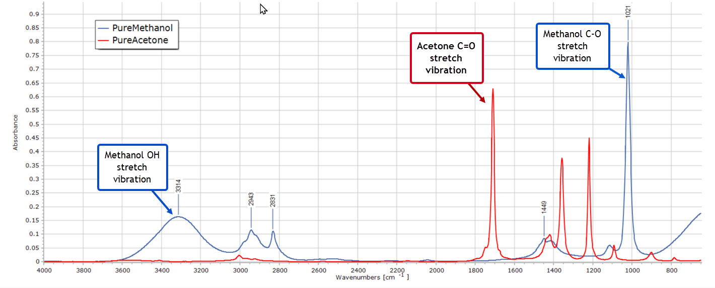
Now you are very familiar with the infrared spectra of the pure solvents methanol and acetone. So you pull up the spectra on your PC display…
Spectra such as these, as you well know, are just very long 2-column lists of numbers. The dependent variable on the vertical axis represents absorbance, fluorescence intensity or some other measured property, and the independent variable on the horizontal axis represents wavelength or wavenumber. Obviously the graphical representation of a spectrum is the one we are all familiar with and is far more visual. But all the information is contained in those myriad data points and they can be processed mathematically. More importantly, well established statistical methods can be applied to this type of data.
The Experimental Design
To assist in solving the contamination problem, you realise that an experimental design is called for. This will consist of the pure solvents of methanol and acetone, plus a series of mixtures of the two solvents in different proportions. These will represent known standards that can be used for calibration purposes.
You then create the design in spreadsheet software as follows:
Sample No
% Methanol
% Acetone
Purpose
1
100
0
Pure Standard
2
98
2
Calibration
3
96
4
Calibration
4
94
6
Calibration
5
92
8
Calibration
6
90
10
Calibration
7
85
15
Calibration
8
80
20
Calibration
9
60
40
Calibration
10
50
50
Calibration
11
40
60
Calibration
12
20
80
Calibration
13
0
100
Pure standard
The numbers are the % amounts of each solvent by volume. Any differences in density between these very similar solvents will be negligible, so you are justified in using % volume when small quantities of the test mixtures are prepared.
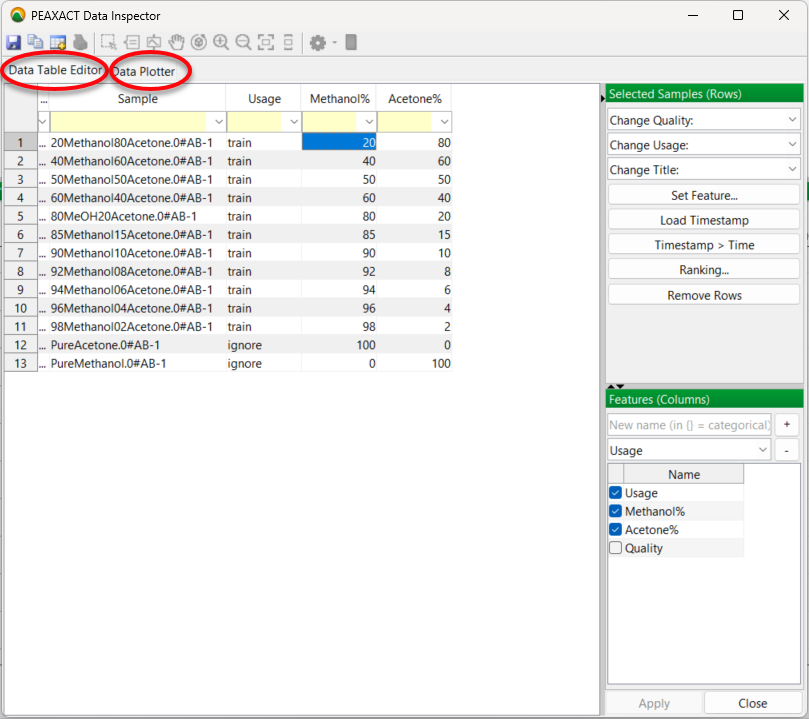
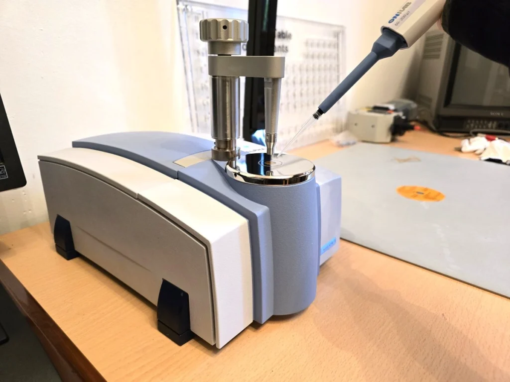
So its over to the lab to prepare these 13 samples and record individual infrared spectra for each sample. This doesn’t take too long with an FTIR spectrometer and ATR accessory. Then you input the spectra into PEAXACT. The software automatically recognises the spectrum files as coming from a Bruker Alpha spectrometer with its native OPUS software. The spectral data import is performed smoothly without any further treatment. You now have all your spectra in PEAXACT and the data is listed in the app’s Data Table Editor:
The data table has a “usage” column added. This is simply a label indicating the purpose of each sample. Mixture samples will be used to calibrate the model and PEAXACT has labelled these “train” for training samples. They are used to train the model.
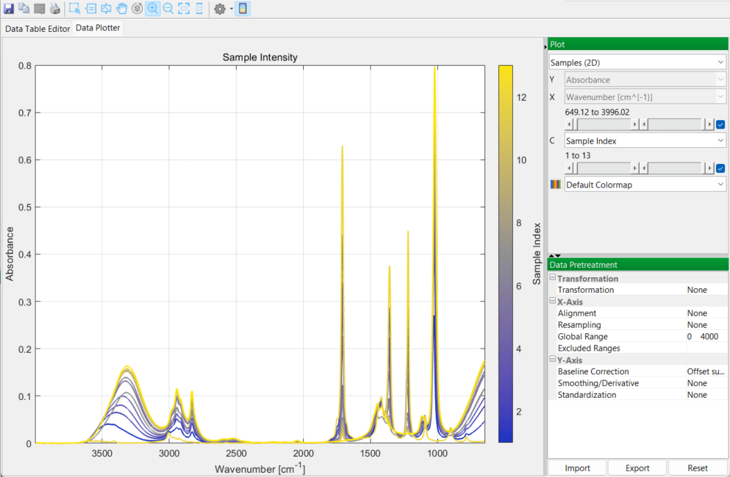
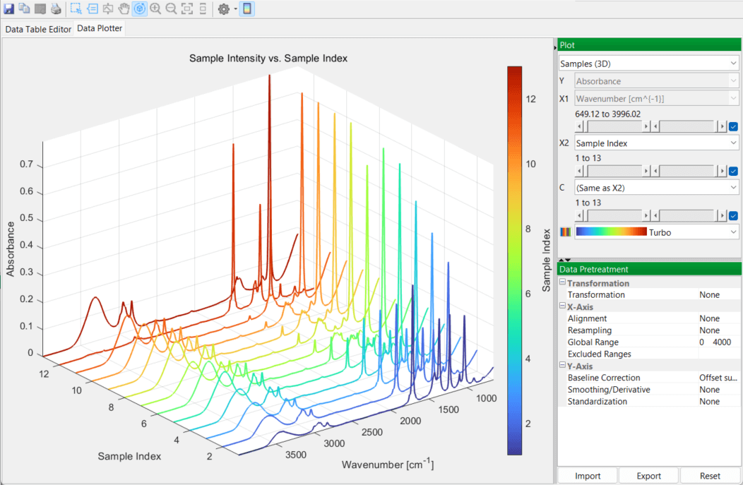
You then switch over to the DataPlotter tab to inspect the various spectra, in 2D and 3D plots:
Creating Models in PEAXACT
You know that the objective is to set up a statistically valid empirical model that will be able to accurately predict acetone contamination levels for future methanol batches. And the goodness of fit of this model will have to be verified when you come to validate the model.
But first of all, you need to create separate models for the two pure solvents, before considering any mixtures. You recall that the PEAXACT training instructor emphasized that the central element in the software is the concept of a model, and the app creates different models that correspond to each stage in the data analysis process.
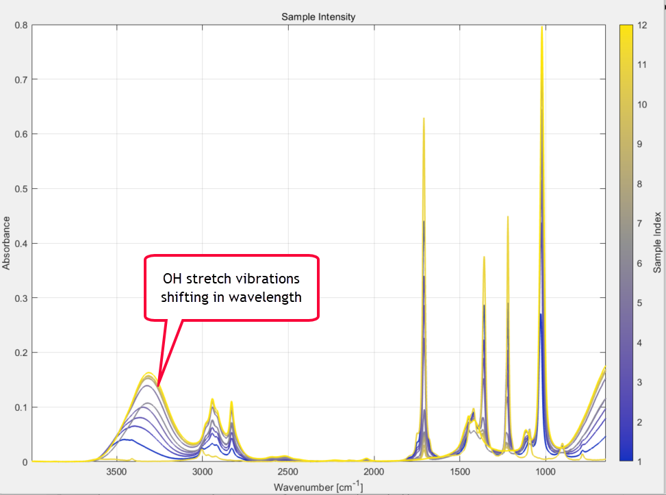
Of immediate concern to you right now is the broad O-H stretching region from 3000-3600 cm-1 of the methanol samples, which is well known and due to hydrogen bonding. The strength of these methanol absorption bands falls as the concentration of methanol in the sample decreases (as expected of course) but the actual wavenumber position of the bands is also changing as the methanol/acetone ratios change. This is caused by different degrees of H-bonding between acetone and methanol molecules as the concentration ratios change. It is clearly visible in the 2D plot of the spectral series that you zoom in on:
It is possible that this could affect any future model performance and goodness of fit, if you attempt to create a model that includes this complex and shifting OH region and also covers the whole spectral range from 360 to 4000 cm-1.
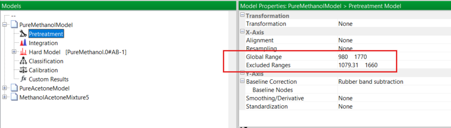
Fortunately, you know from the overlaid spectra of the two pure solvents that there are two well isolated IR absorption peaks, one at 1700 cm-1 and one at 1021 cm-1 without other overlapping peaks. You recognise these as the C=O stretching vibration of acetone and the C–O stretch from methanol, respectively. So in the Pretreatment menu of PEAXACT you modify the global range for the model, limiting it to be from 980 to 1770 cm-1. Also, you exclude the range from about 1080 – 1660 cm-1, as depicted here:
Pure Solvent Models
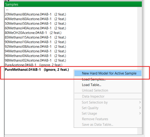
Now it’s time to start building models, starting with the pure solvents. You know from your previous training that the easiest way to create a new model for a pure component is to right-click on the relevant one in the Samples Panel. For methanol, this is shown here:
This new model is created and added to the Models Panel with the name of the sample (in this case PureMethanol) that you used. PEAXACT refers to these models as “hard” models. (A hard model in chemometrics is a model that is grounded in the laws of physics and chemistry and not just “patterns in data”. A good example would be to model absorbance using the Beer-Lambert law.)
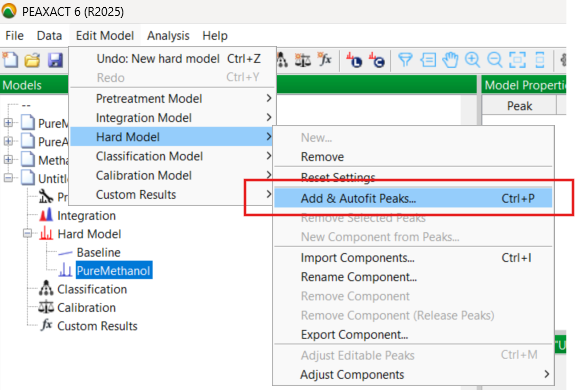
At this point, you know that the newly created model is really only a sort of place holder, requiring editing and further development. This development takes the form of fitting a number of curves to simulate as much as possible the true absorption peak seen in the spectrum. So you go in the Edit Model menu, and under Hard Model, you select “Add and Autofit Peaks”:
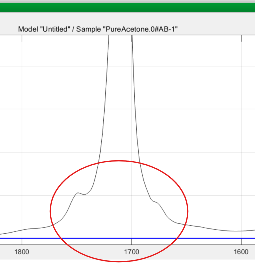
PEAXACT then asks you for the number of peaks to be added, the default being one. You know from training that it is best to add a reasonable number of peaks. Even for a single measured absorption band, several model peaks may be needed to adequately model the complete envelope of the true peak. A good example is the 1700 cm-1 band of acetone which has “wings” or “tails” in the measured spectrum, clearly shown below, and you need to include these:
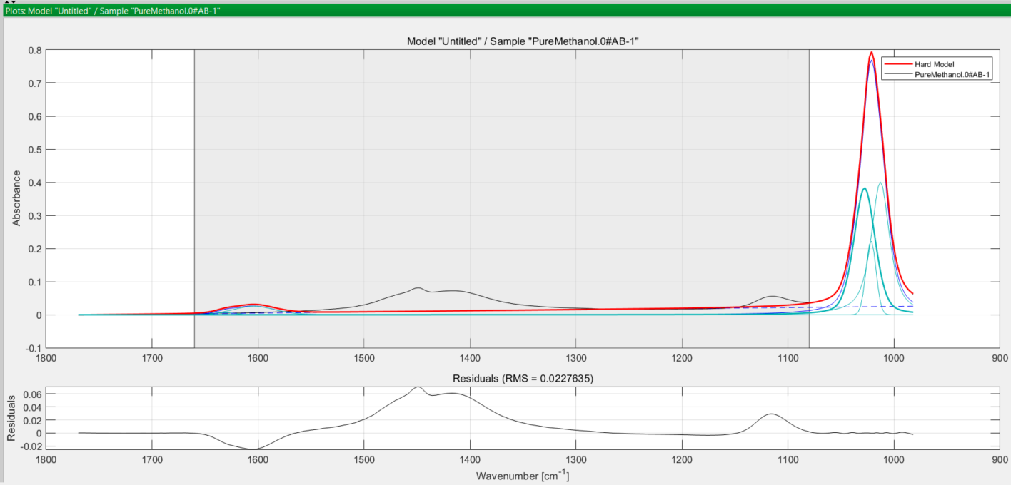
A choice of about 5 for methanol is reasonable, since you have restricted the model range at the Pre-treatment stage earlier. You select 5 and the software fits the peaks to the true peak in the spectrum as you see here:
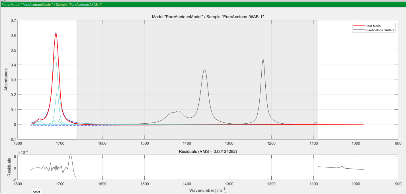
You save this methanol hard model, then move on to consider acetone. Performing the same steps for the acetone model, you obtain the following set of curves:
In both cases, the turquoise coloured curves are the peaks used to model the true (observed) absorption peak in black, and the thicker red curve is the final modelled peak. The greyed-out area in both spectra is the excluded wavenumber range you defined earlier at the pretreatment step.
Now it is time to create a Mixture Model using the models of these two pure components you have just created, together with the different mixture samples of the experimental design.
Creating the Mixture Model
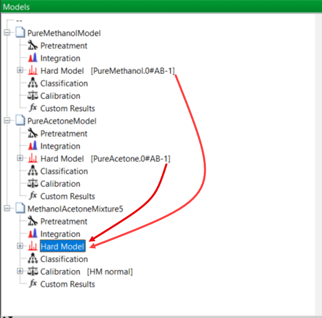
From your previous training, you know that the easiest way to create the mixture model is simply to open the model “tree” for each of the pure components, methanol and acetone, and drag and drop each pure component model into a new model representing the mixtures. This new mixture model is then saved:
Creating the Mixture Model
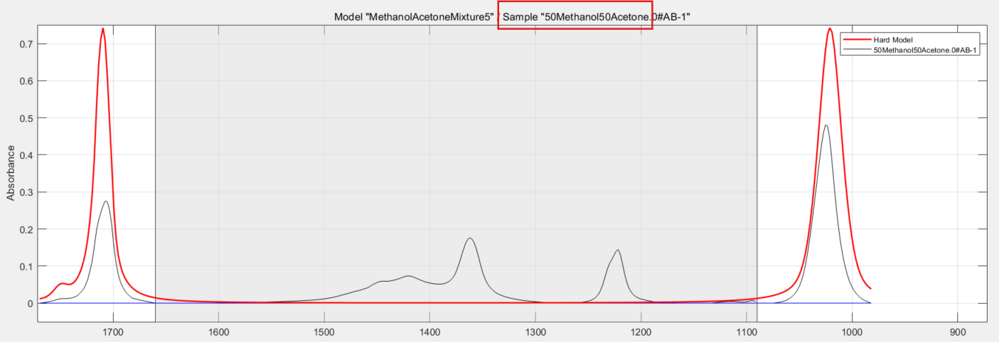
The end result is this series of curves:
You know that the black trace is an actual recorded spectrum of one of the training samples, in this case it is a 50/50 mixture of methanol and acetone (red box). The thicker red line is the mixture model itself, used for all of the calibration samples. And again, the greyed out region is the excluded range you defined at pretreatment.
Now it’s time to check calibration and goodness of fit of this model to the actual spectra of the various solvent mixtures of the experimental design. This is carried out by running a calibration model.
Calibrating the Mixture Model with the Training Samples
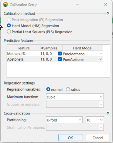
To set up the calibration, you use a Hard Model Regression with the predictive features of the pure solvent models you created earlier for both methanol and acetone. As for the regression settings, it’s best to select cubicas the maximum function for the least squares regression. This can always be changed later if a cubic polynomial equation “overfits” the data, which you want to avoid.
Calibration Setup Settings
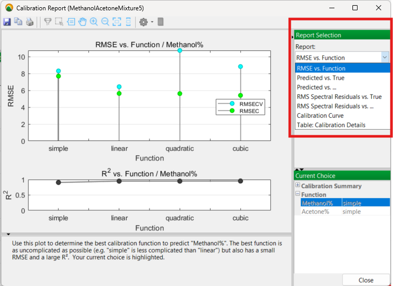
The calibration process is then run with the full set of 11 mixture samples and produces the following results with the mixture model you created in a visual Calibration Report:
The initial Calibration Report output
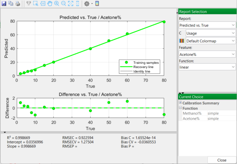
Prior to selecting a final mixture model to apply, there are a number of options to examine in this report, especially the Predicted vs. True and the Calibration Curve outputs. The RMSE (Root Mean Square Error) for each model function (linear, quadratic, cubic) is also considered.
Linear Model
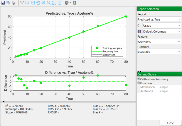
Quadratic Model
The Calibration Curve outputs generate very similar and promising results. Acetone curves for both linear and quadratic models produce excellent results with high R2 values greater than 0.99. A cubic model is very slightly higher in the degree of fit; however you are sensitively aware of the downfalls of over-fitting the model to the real data. So you accept a quadratic model as being the best choice. Once accepted, PEAXACT will use a quadratic model in the next and final stage of the whole process…
This is validating the model with some new samples to test the model’s predictive capability.
Validating the Model
In order to validate the Mixture Model, you know that you need some additional samples. These samples will resemble, but not equal, the ones used in the earlier experimental design. So they will be similar to the concentrations used previously.
You deliberately make up more samples that have small quantities of acetone, relative to methanol, clustered together. After all, you are dealing with a contamination problem here with probably very low levels of acetone. That being said, it is also prudent to cover the whole range of proportions. So a second spreadsheet is prepared with the following values:
Sample No
% Methanol
% Acetone
Purpose
14
99
1
Validation
15
97
3
Validation
16
95
5
Validation
17
93
7
Validation
18
91
9
Validation
19
89
11
Validation
20
87
13
Validation
21
84
16
Validation
22
70
30
Validation
23
65
35
Validation
24
55
45
Validation
25
45
55
Validation
26
35
65
Validation
27
25
75
Validation
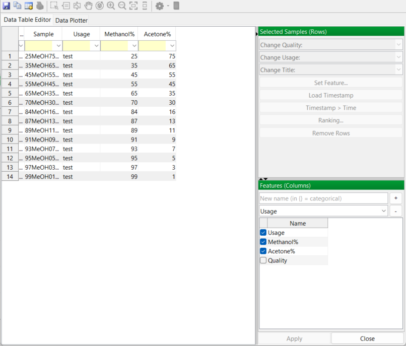
Off to the lab again to make up these 14 samples and run the spectra. The 14 spectrum files are then imported into PEAXACT as before and the new list of samples is added to the Data Table Editor. The application again creates a usage column in the data table and you identify all samples as “test” for future reference, since these are the validation samples:
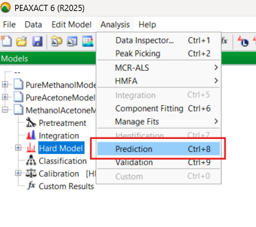
In the software, you pull down the Analysis menu choices and select the Prediction routine:
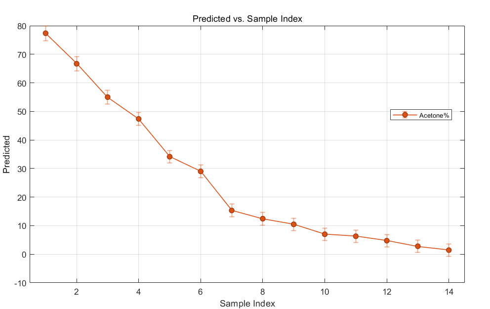
The software processes the new spectrum data and produces several plots. Focusing on acetone levels, you briefly examine the chart of the predicted values versus sample number. The error bars are encouragingly tight.
You next move on to the Validation routine in the drop-down Analysis menu. After running a validation model, a number of very useful plots are generated:
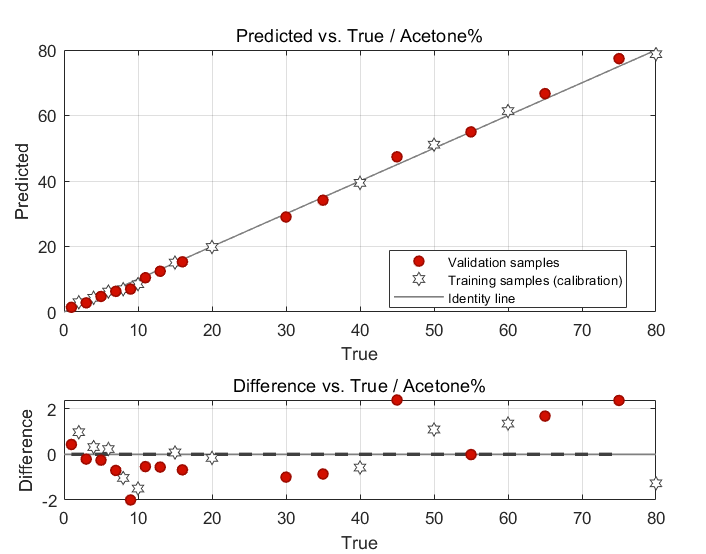
This appears to be the important result. The “Predicted vs. True Value” graph demonstrates that the predictive ability of your chosen mixture model performs very well. Differences between model-predicted values and true (observed) values are small and reported in the chart. Both training samples used in the calibration and those of the validation (test) samples all lie nicely on the identity line:
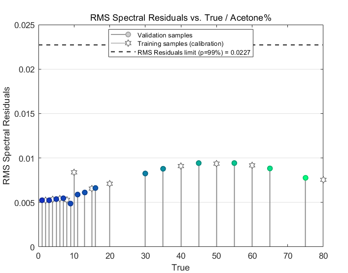
A brief look at the residuals confirms the goodness of fit of the model to the spectrum data:
These values, all of which are less than 0.01, are much lower than the dotted line limit of 0.0227 at a confidence level of 99% that you see in the chart. Basically, the lower the residuals are here, the better the model is at fitting the data at a statistical confidence level of 99%.
There are a few more graphical results that you briefly examine, and all confirm that the quadratic Mixture Model you selected will perform well and do a good job at predicting any future levels of contamination by acetone. Satisfied with all the data processing and analysis, you save all your PEAXACT files.
The fun part is over for you in the role of “data analyst”. You now have the somewhat less interesting, but still very important, job of writing up the SOP to support your colleagues in the QC department!
Final Scenes...
You spend the next couple of days writing the SOP, using the company’s official documentation software and format. You explain the methodology, procedures, results and conclusions including screenshots taken during the analysis. The procedure is then submitted to the company’s QA (Quality Assurance) organisation for review and approval. After a few back and forths with QA, correcting various typos in the text, revising the procedure and adding additional explanations requested by QA, the SOP is finally approved, and it becomes official. The SOP is then passed on to the QC department for implementation.,
Finally, and with the approval of your R&D manager, you send an email to the head of the QC department with a copy of the SOP together with a recommendation that the QC department looks into purchasing a license for PEAXACT software, that it contacts the company and arranges for some on-site training of QC staff.
Satisfied with the contribution you have made, you can now get back to your own R&D projects that have been on the back-burner for far too long.
(Meanwhile, those Process Engineers in the manufacturing plant are still working overtime trying to identify the actual source of the original acetone contamination …. but that’s an entirely different story! 😉)
Afterword...
Although purely fictional, this story of how an industrial process contamination problem can be evaluated and analysed by chemometrics techniques is nevertheless very relevant and important for scientists and engineers working in industry.
This specific example, using a methanol-acetone system, was deliberately selected because the pure component spectra possess strong and isolated IR vibrational bands. These can be analysed relatively straightforwardly using chemometric methods and a hard model. Real-world problems of mixtures of this type are often more complex and not as clear-cut, but several other chemometrics techniques exist, not mentioned in any detail here, that can assist in solving these problems in a statistically relevant manner.
Even with this simple two-component system described in the story, it is clear that some pre-processing of the data, prior to any model creation, was an important first step in the whole process. In doing so, a practical and useful model, with statistically proven predictive capability, was able to be developed and then implemented.
Not mentioned in the above scenario, for example, is the fact that if a mixture model had been created that had used the full spectral range for the samples, the goodness of fit of the model would have deteriorated significantly, owing to those shifting OH absorption peaks in the different samples, as well as other overlapping bands mentioned in the story. This demonstrates the importance of carefully considering spectral characteristics at the pre-treatment stage, whatever the software you happen to be using.
Acknowledgement
I am most grateful to Dirk Engel at the S-PACT Company for various discussions. Dirk is one of the co-creators of PEAXACT, and provided much useful advice and guidance with very prompt messages back to me, when I was learning how to use the software.
On a personal note, although I taught experimental design methods in several companies during my own R&D career, that was over 25 years ago! Chemometric methods and software have both moved on very considerably since that time in terms of user friendliness!
There are several chemometrics software packages out there, but in my opinion PEAXACT is one of the better ones. The logical steps of model pretreatment, creation, calibration and validation are well explained in online tutorials. The app is highly interactive and visual in its approach to chemometrics data processing and analysis, especially when it comes to examining spectroscopic data. Highly recommended.
References
S. N. Deming and S. L. Morgan, Experimental Design: A Chemometric Approach, Elsevier, 1987.
J. N. Miller and J. C. Miller, Statistics and Chemometrics For Analytical Chemistry, Pearson Education Ltd., 2000.
R. G. Brereton, Chemometrics: Data Analysis for the Laboratory and Chemical Plant, Wiley, 2003.
Introduction The historical development of the infrared spectrometer was described in a three-part article a few months ago. A table was presented that listed the…