Introduction
Here’s what happens when a highly fluorescent compound, in this case sodium fluorescein, dissolves in water and a UV lamp shines on the solution:
The above video shows fluorescein to be a highly fluorescent molecule. But what is curious, and somewhat odd, is that this strong fluorescence would have been even stronger if it wasn’t for the water! The presence of water molecules are, in fact, reducing the fluorescence from the fluorescein, and substances that do this are called fluorescence quenchers.
In this article, two simple experiments the home scientist can try that demonstrate these effects are described. One involves the quenching of fluorescence of sodium fluorescein by potassium iodide (KI) and the other the quenching of quinine fluorescence by chloride ions (table salt).
But first, here’s a little more detail on fluorescence quenching…
Fluorescence Quenching
In general terms, fluorescence quenching is defined as any process that reduces the intensity of fluorescence from a molecule in solution. Several chemical compounds can do this and, as mentioned above, they are known as quenchers.
If you are not quite sure what exactly fluorescence is in scientific terms, a basic introduction is provided in this post. This link also describes other photophysical and photochemical processes that can compete with a fluorescing molecule. A fluorescent molecule contains a chemical functional group that can be regarded as its production centre. This light emitting group within the structure of the molecule is called the fluorophore.
In photochemistry, a reduction in fluorescence intensity is caused by a variety of mechanisms. The most common one is called collisional quenching. As the name implies, this happens when a molecule in an excited state is deactivated (loses energy) upon collision with some other molecule in solution, which is termed the quencher. As a result, the excited molecule drops to a lower energy state (usually the lowest energy or ground state) after its encounter with the quencher.
Expressing this as a very simple chemical equation we have
A* + Q → A + Q
where A is the fluorescing molecule, Q is the quencher and * denotes an excited energy state. An alternative expression could well be
A* + Q → A + Q*
where the quenching molecule itself becomes excited during the encounter and could itself then fluoresce, at some wavelength, or could be de-activated by a radiationless process.
A large number of molecules can act as collisional quenchers. Water is a good example as we saw in the video above. Other common quenchers include oxygen, the halide ions such as bromide (Br–) and iodide (I–), various amines and also electron deficient compounds such as acrylamide. The actual mechanism of quenching depends on the fluorophore-quencher pair. For example, the quenching of the fluorescence of indole (a molecule that is often used in making perfumes) by the quencher molecule acrylamide occurs by electron transfer from indole to acrylamide.
Fluorescence quenching by halogens and other so-called “heavy” atoms takes place through a mechanism known as spin-orbit coupling. This is a photophysical process that induces intersystem crossing to the triplet state. If any of these terms are unfamiliar, a useful explanation is provided in this article.
The amount of collisional quenching depends on temperature, since increasing the temperature increases the kinetic energy of the molecules in solution and consequently the likelihood of more collisions. This explains why some experiments performed to measure fluorescence, and also phosphorescence, are often carried out at low temperatures in order to minimize quenching.
In addition to collisional mechanisms, the quenching of fluorescence can occur by other processes. Fluorophores can produce non-fluorescent complexes with quenchers. This is known as static quenching because it occurs in the ground state, with no light absorption involved, and does not rely on molecular diffusion or collisions. And quenching can also occur through the attenuation of the incident light by the fluorophore itself, called self-quenching, or through some other light absorbing species.
We now move on to consider the first practical example: the quenching of quinine fluorescence by sodium chloride (NaCl).
Example 1 - Quinine Fluorescence Quenching
In a previous post we used fluorescence spectroscopy to determine the amount of quinine present in a popular can of tonic water. Here, we are going to see how quinine fluorescence is quenched by a halide ion – sodium chloride or common table salt.
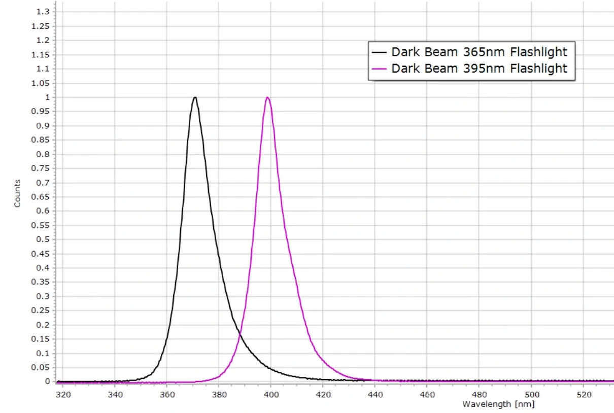
Sources of pure quinine crystals or quinine sulphate can be found online. Alternatively, you can use a can of tonic water. The UV light source used in the tonic water video is a common Black Light. These are small flashlight-sized lamps which are readily available online. They are popular for detecting urine stains if you have a dog or a cat around the home. A lamp that emits a fairly broad band in the region 350 – 400 nm is a good choice. Emission spectra from two types of black lamps can be seen here:

We could perform this experiment with just a sample of tonic water. But in this demonstration, we will use pure crystals of quinine free base. Quinine itself is only sparingly soluble in water, so we dissolve quinine in dilute sulphuric acid (H2SO4) which converts quinine to the salt quinine sulphate, a more soluble form. And we use common table salt (NaCl) as the quencher, for its source of chloride ions Cl–. Ordinary table salt actually contains trace amounts of sodium iodide, typically around 1700μg iodide per 100g of salt. Since iodide ions are also quenchers there will be a minute contribution from iodide quenching in this demonstration; but by far the largest contribution to the quenching of quinine fluorescence comes from chloride ions.
Solution Preparation
If you want to try this experiment yourself some common laboratory glassware such as volumetric flasks and pipettes are needed. These are available online, either new or used, at reasonable cost.
Stock Solutions
The simplest, most reliable and accurate method for preparing the various solutions is to start from stock solutions of quinine and sulphuric acid. The common solvent will be 0.1M H2SO4. The acid is available from drugstores and is typically 15% concentration, which is equivalent to 1.68M (M = Molar or moles per litre). So this needs to be diluted with DI water to produce a stock solution of 0.1M which will be used for all our solutions.
For the quinine stock solution, a good starting concentration is 10-3M. Since the free base of quinine is being used here, the molecular weight is 324.43g/mol. A useful practical volume for quinine stock solution is 100mL, therefore we use 32.443 mg of pure quinine and dissolve this in 100mL of our 0.1M sulphuric acid. This stock solution needs to be protected from light so aluminium kitchen foil wrapped around the flask is useful here.
For the sodium chloride stock solution, we prepare a 1M solution in 0.1M H2SO4. The molecular weight of NaCl is 58.44 g/mol and, as with the quinine stock solution, we dissolve 5.844 g of the salt and make the solution up to a volume of 100 mL with 0.1M acid.
In this way, the ionic strength of the acid is constant across all solutions once we spike the quinine with NaCl.
The Measurement Solutions
For the measurement solutions, a useful practical range to study these quenching effects is 0, 0.005M, 0.01M, 0.015M, 0.02M and 0.025M NaCl. Since we will be using 1cm square spectrometer cuvettes, only relatively small volumes of the test solutions are required, typically 10mL. So 10mL volumetric flasks are used.
For each test solution in a 10 mL flask we add 100 μL of the 10-3 M quinine stock solution followed by quantites of the NaCl stock solution according to the following table:
| Target NaCl Concentration [M] | Volume of NaCl (microlitres) |
|---|---|
|
0.000 |
0.0 |
|
0.005 |
50 |
|
0.010 |
100 |
|
0.015 |
150 |
|
0.020 |
200 |
|
0.025 |
250 |
Recording the Fluorescence
The experimental setup is identical to that used in the tonic water demonstration and is provided again here for reference:
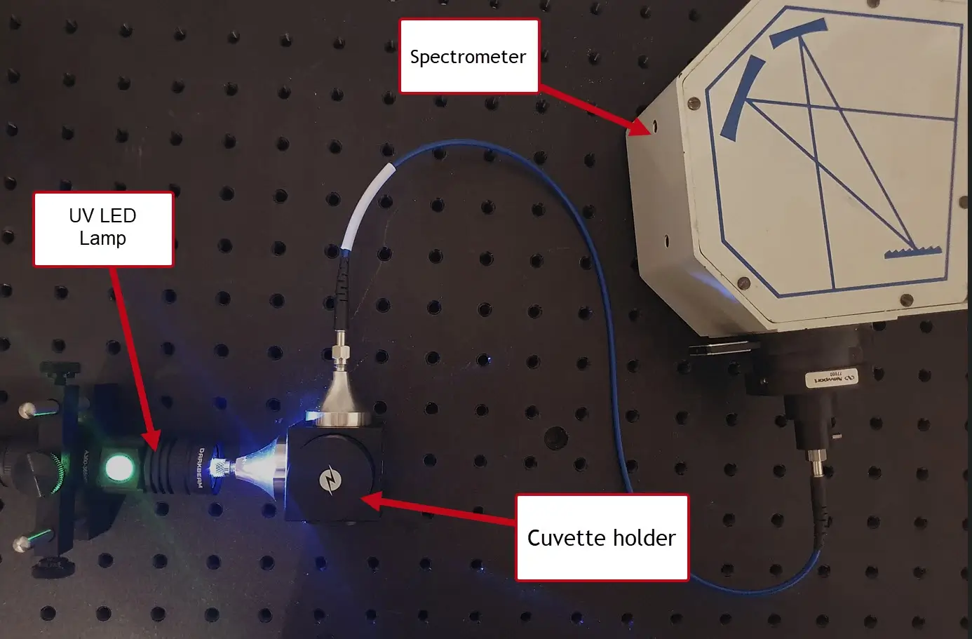
Fluorescence spectra for all six solutions were recorded with the setup shown above and are produced below. Any spectrometer can be used, such as the popular “hand held” versions from companies such as Ocean Optics, Thunder Optics or other manufacturers. The fluorescence intensity on the vertical axis at or close to the maximum on the light emission curve (λmax) is recorded.

The Stern-Volmer Equation
In order to continue analyzing the spectra, we apply the Stern-Volmer equation. This is a very useful expression describing the kinetics of fluorescence quenching via a collisional mechanism. It was proposed over a hundred years ago in 1919 by Otto Stern, a German-American physicist, and Max Volmer, a German physical chemist. And the relationship is still very applicable today. It is from this expression that we can determine the rate constant (a measure of the speed of any chemical reaction) for the quenching process.
The Stern-Volmer equation describes the kinetics of collisional quenching between the quencher molecule and the fluorophore, and is given by
F0/F = 1 + KSV[Q] = 1+ kq τ0[Q].
F0 is the fluorescence intensity measured without quencher, F is the intensity in the presence of quencher, KSV is the Stern-Volmer quenching constant and [Q] is the quencher concentration in moles per litre. kq is the bimolecular quenching constant (that we want to determine) and τ0 is the fluorescence lifetime of the fluorophore in the absence of any quencher.
A graph (usually called a Stern-Volmer plot) of the ratio of the two fluorescence intensities F0/F plotted against quencher concentration [Q] will produce a straight line with a slope equal to KSV and an intercept on the Y axis equal to 1. Alternatively, we could plot (F0/F – 1) against [Q] in which case the line passes though the origin. This graph is shown here:

To proceed further, we need the fluorescence lifetime τ0 of quinine in dilute sulphuric acid. An often cited literature value at room temperature is 19 – 20 ns. So a value of 19.5 ns is used in these calculations.
KSV, the Stern-Volmer constant, is equal to the slope in the above plot and is ≅ 190 M-1. This value is appreciable, indicating strong dynamic (collisional) quenching by the chloride ions from the salt solution.
From the Stern-Volmer equation, kq = KSV / τ0
Knowing KSV, we can now calculate kq, the bimolecular rate constant for quenching:
KSV = 9.72 x 10⁹ L mol-1 s-1.
This value is very close to the diffusion-controlled limit in aqueous solution, which is around 1010 L mol-1 s-1. So this value is consistent with efficient collisional quenching.
Example 2 - Quenching of Fluorescein Fluorescence
Fluorescein belongs to the family of dyes called the Xanthene dyes whose general core structure is shown here:

Xanthene itself is not particularly interesting, but its derivatives form some very useful synthetic dyes such as the Rhodamine and Eosin dyes as well as the Fluorescein family of dyes. The sodium salt of fluorescein has the following structure:

It is readily soluble in water and fluoresces intensely under UV light as we saw in the above video. In order to observe fluorescence quenching with this system, an entirely similar methodology to the above quinine example was used.
A series of fluorescein sample solutions were prepared and then spiked with different concentrations of potassium iodide, in the same way as those prepared for the quinine experiment.
Fluorescence spectra for each solution were then recorded as before, using the same experimental setup. This produced the following set of fluorescence spectral curves, in this case the fluorescence spectra exhibiting a λmax at 525 nm in the green-yellow region of the visible spectrum:

Values of fluorescence intensity at the λmax of 525 nm were recorded and the following Stern-Volmer plot produced:

In the above graph, F0 / F has been plotted against concentration, as opposed to F0 / F – 1 for the quinine case (just to change things a little!) In this case, the line should pass through 1 on the vertical axis, or be close to it, within experimental error. And this is indeed the case, with the intercept equal to 0.964. This confirms that the quenching process is primarily collisional (dynamic) quenching. Since the Y intercept is not exactly = 1, there may be some contribution from static quenching, although the difference is very small and the uncertainty may be due only to experimental error.
In this example, the Stern-Volmer constant KSV ≈ 10 M-1 from the slope of the line, which is consistent with a diffusion-limited dynamic quenching process, although significantly lower than the case with the quinine example.
Using a typical literature value for the fluorescence lifetime τ0 for sodium fluorescein of 4 ns in aqueous solution, we can compute the quenching rate constant kq for this system as
kq = KSV / τ0
Thus kq = 9.96 M-1 / 4.0 x 10⁻⁹ s-1 or
kq = 2.49 x 10⁹ L mol-1 s-1
In Conclusion
This was a longer post than usual, but it does give the reader some insight into an important standard technique employed in the photochemistry and photophysics of organic molecular systems.
The method assists researchers in studying the kinetics of the various processes that can take place when light emission from organic molecules is reduced (quenched) by other molecules in such systems and rate constants for these reactions can be measured.
References
- J. R. Lakowicz, (2006), Principles of Fluorescence Spectroscopy, 3rd Edn., Springer.
- B. Valeur, (2001), Molecular Fluorescence: Principles and Applications, Wiley-CH.
From Steve’s Open Lab