Introduction
A number of articles at Steve’s Open Lab have demonstrated how the home experimenter can detect fluorescence from different samples and from there to record a fluorescence (emission) spectrum. How fluorescence is defined in scientific terms was explained in one of the very first articles on this site if you need a quick refresher. A number of more recent articles went on to look at fluorescence in luminescent minerals, in measuring the quantity of quinine contained in a popular can of tonic water, and in determining the quantity of riboflavin in a vitamin supplement tablet. All of these demonstrations used a very simple experimental setup and optical path of
Light Source → Sample → Spectrometer
with flexible optical fibres directing light from the excitation source to the sample and then guiding fluorescent emission from the sample to a spectrometer. This is a very basic setup and works well with the examples mentioned above. In this article I want to move on significantly to the next degree of sophistication and to consider a commercial instrument.
The Professional Fluorescence Spectrometer
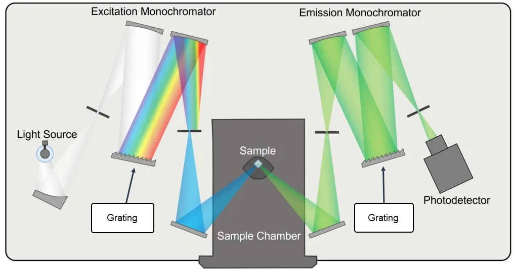
A commercial fluorescence spectrometer is called a spectrofluorometer or spectrofluorimeter. The two names are entirely synonymous and only reflect regional naming differences used by the scientific community. A simplified schematic view of the inside of a spectrofluorometer is shown in Fig. 1.
Main Components
The instrument consists of a broad-band UV light source, two monochromators, a sample chamber, and some form of photodetector. The light source most widely used is the xenon arc lamp, since it provides strong and broad light emission across much of the UV and visible spectrum. The two monochromators are optical devices in their own right, and two are integrated into a modern spectrofluorometer, one on the excitation side and one on the emission side. The function of the excitation monochromator is to select and isolate a specific wavelength from the large choice of wavelengths offered by the xenon arc lamp. The grating disperses all wavelengths from the lamp and a very narrow wavelength band is selected. Only this passes through the exit slit of the excitation monochromator and on to the sample compartment.
After the sample absorbs excitation light, it emits fluorescence at longer wavelengths. This emission is observed at 90° from the excitation light beam. Fluorescent light emission from the sample is usually spread over a range of wavelengths which are characteristic of the sample. This light enters the entrance slit of the emission monochromator. Its role is to separate the emission into its component wavelengths, and to select which wavelengths, in turn, reach the detector by rotating the grating during a wavelength scan. Each wavelength passes through the exit slit of the emission monochromator and on to the photodetector.
The most widely used photodetector in a spectrofluorometer is the photomultiplier tube or PMT. This is a highly sensitive light detector that converts extremely weak light emission into a measurable electrical signal. Fluorescent photons enter the PMT and strike a photocathode (Fig. 2). Each absorbed photon causes the cathode to emit an electron via the photoelectric effect. The electron is then accelerated toward a series of electrodes called dynodes. At each dynode one electron can produce several secondary electrons. The chain of dynodes are held at progressively increasing voltages, each producing secondary electrons within the tube. So there is an increasing cascade of electrons that finally reach the anode to produce a measurable electrical signal. We have a large number of electrons generated through a multiplication process that began originally with one photoelectron.
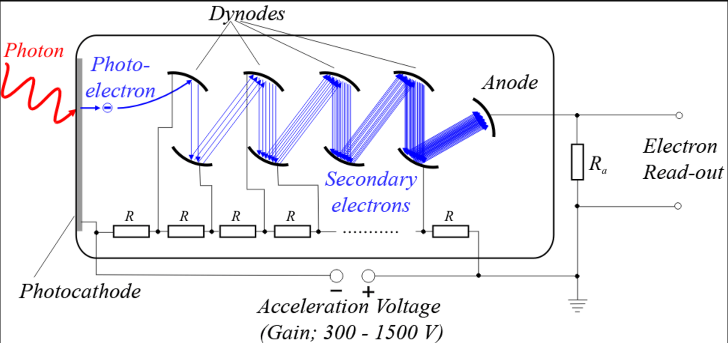
The PMT offers extremely high gain and a fast response time, making it ideal as the photodetector of choice in a spectrofluorometer.
Detailed Optical Layout
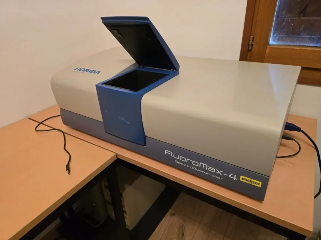
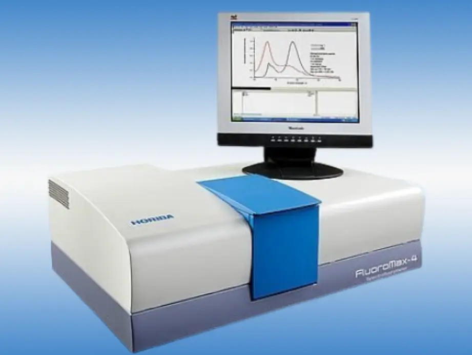
In more detail, Fig. 3 shows the optical layout of a professional spectrofluorometer, using the Horiba FluoroMax-4® instrument as an example.

Legend:
- 1 = Xenon arc lamp and lamp housing
- 1a = Xenon lamp power supply
- 1b = Xenon flash lamp (included only with the P version of spectrometer)
- 2 = Excitation monochromators
- 2a & 2b = Excitation monochromator slits
- 3 = Sample compartment
- 4 = Emission monochromator
- 4a & 4b = Emission monochromator slits
- 5 = PMT and tube housing
- 6 = Reference detector
Technical Specs
With the multiple optical components apparent in Figure 3, it is no surprise that modern spectrofluorometers are usually operated under full computer control. Software can control wavelength scan speeds, control the rate of rotation of gratings on their motorized supports, and adjust and set monochromator slit widths, which are usually expressed as “bandpass” in nm. Monochromator slit widths are continuously variable so as to produce a bandpass from 0 to about 20 or even 30 nm which covers most if not all user applications. Fluorescence spectra under normal conditions are recorded with a bandpass of 1-4 nm for the excitation monochromator and between 1 – 4 nm for the emission monochromator, depending on the spectral resolution required.
A summary table of typical technical specifications is provided below, and taken from the Horiba FluoroMax-4® Operating Manual:
| Component | Comments |
|---|---|
|
Excitation source |
150 W xenon, continuous output, ozone-free lamp |
|
Optics |
All reflective for focusing at all wavelengths |
|
Spectral Dispersion |
4.25 nm / mm |
|
Monochromators |
Czerny-Turner design; f/3.5, 1200 grooves/mm reflection gratings; resolution 0.3 nm; maximum scan speed 80 nm per second; accuracy ±0.5 nm; step-size 0.0625 nm – 100 nm; range 0-950 nm |
|
Detectors |
Calibrated photodiode for excitation reference correction from
200–980 nm.
Emission detector is an R928P for high sensitivity in photon counting mode (200–850 nm). High voltage = 950 V, linearity to
2E6
counts s–1
, < 1000 dark counts s–1
. |
|
Sensitivity |
Typically S/N = 3000:1 for DI / HPLC grade water for a water-Raman scan at 397 nm, with a bandpass of 5 nm, 1 second integration time.
|
|
Excitation Shutter |
Computer/software controlled |
|
Integration Time |
Variable from 0.001 s to 160 s |
|
Slit Widths |
0–30 nm bandpass, continuously adjustable via host computer |
Producing a Spectrum
The usual requirement in the lab is to obtain the Emission Spectrum. This is the “normal“ fluorescence spectrum, and is obtained when we select and fix the excitation wavelength of the light source, keeping it constant, and we scan the wavelengths emitted by the sample with the emission monochromator. The resulting trace is a representation of the distribution of fluorescent light emitted at different wavelengths.
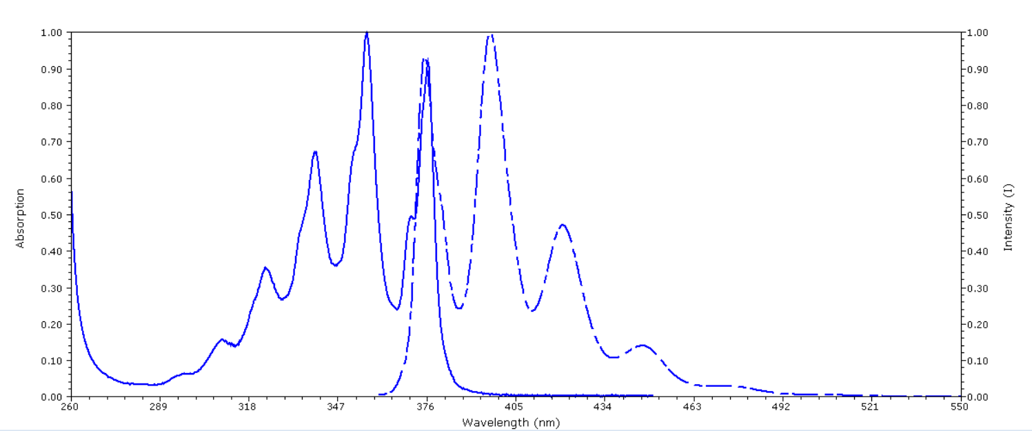
Alternatively, we could set up the instrument to record the Excitation Spectrum. This closely resembles, but not identical to, the actual absorption spectrum. It is the case where a fluorescence emission wavelength is first selected and kept constant, and the instrument changes the wavelength of UV excitation light using the excitation monochromator and slit. As an example, consider this representation of an emission spectrum of an organic molecule in Fig. 4A that possesses several emission bands:
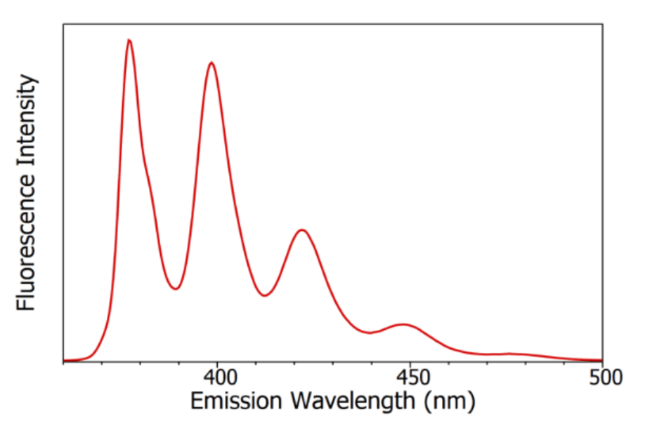
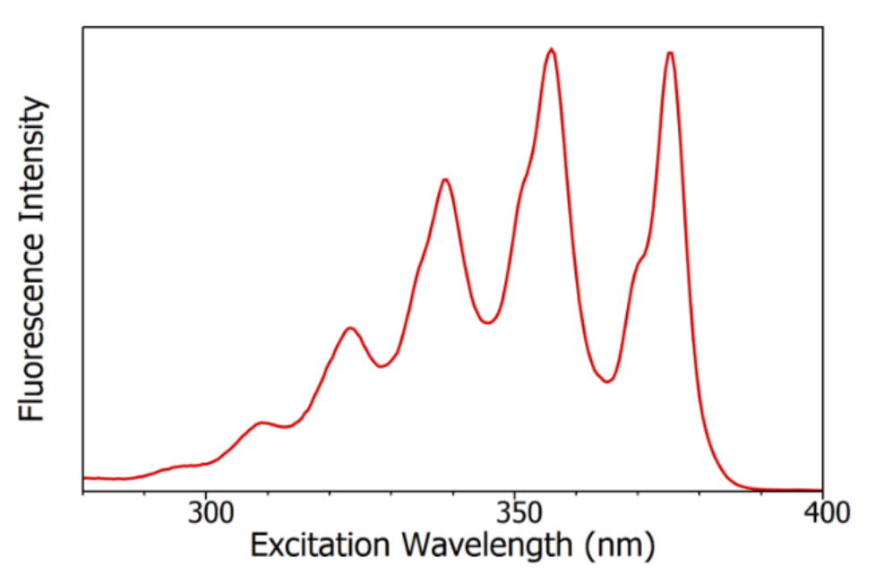
We can select a strong emission band in Fig. 4A, for example the one close to 400 nm. The emission monochromator slit is kept fixed at this wavelength. If we then scan the range of excitation wavelengths from, say, 250 nm to 400 nm, we obtain the excitation spectrum (Fig. 4B).
A real-life example is shown below for the polynuclear aromatic hydrocarbon anthracene dissolved in cyclohexane. (Taken from the PhotochemCAD database.)
Final Words...
This is just one configuration of a professional spectrofluorometer, and represents the “classical” wavelength scanning design. Still widely used, still very important. Another design is to replace the emission side monochromator with a CCD detector. This eliminates the need to perform an emission wavelength scan, which does take several seconds, even minutes, depending on the spectral resolution required. With CCD detection, all wavelengths are detected simultaneously, so we obtain a spectrum virtually instantaneously. This is parallel photon detection, relative to sequential detection. The big advantage is speed, making the instrument particularly powerful for fluorescence kinetics, photobleaching experiments and similar studies. And it is particularly rapid when we want to produce an EEM of a sample. Good examples are the Horiba Duetta and the Edinburgh Instruments FLS1000.
Although tempting to conclude that CCD detection is better, this is not necessarily true. CCD detection comes with increased read noise, dark current and variable spectral response. If high sensitivity for very weak fluorescence emitters is needed, then the tradtional design with a PMT wins the day.
A future article will recount how I was able to acquire a second-hand Horiba FluoroMax-4® spectrofluorometer for Steve’s Open Lab and to get it up and running.