Introduction
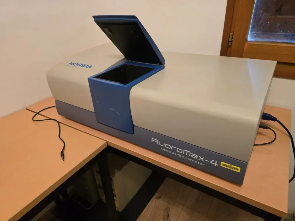
In a recent article on the commercial fluorescence spectrometer, the concepts of the excitation spectrum and the emission spectrum were explained. Very briefly, the excitation spectrum displays the wavelengths of light that a molecule absorbs to become promoted to a higher energy state, while the emission spectrum shows the wavelengths of light the molecule releases as it drops back down to a lower energy state. While briefly in the higher energy state, very rapid picosecond processes such as vibrational relaxation cause the molecule to lose energy before it has time to emit light again. This means that the emitted light (fluorescence) always has a lower energy than the light originally absorbed. This shifts the fluorescence/emission spectrum to longer wavelengths compared to the excitation spectrum. This wavelength shift is called the Stokes Shift, after the Irish physicist G. G. Stokes.
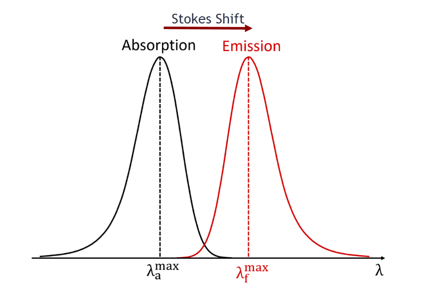
In practical terms in a real experiment , the emission spectrum is obtained by keeping an appropriate excitation wavelength constant and then scanning the emission monochromator over a range of longer wavelengths. In the same way, the excitation spectrum can be recorded by keeping an emission wavelength constant and then scanning the excitation monochromator over a suitable range of shorter wavelengths.
The obvious next question is this… what happens if we scan both monochromators simultaneously? What happens when we systematically record a whole sequence of emission spectra across a stepwise range of excitation wavelengths?
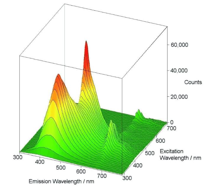
This “dual scan” approach has become a popular technique with modern spectrofluorometers, since it was introduced by Gregorio Weber in 1961. The procedure collects a huge three-dimensional dataset composed of an excitation wavelength series, an emission wavelength series and fluorescence intensity for each and every incremental wavelength setting. This dataset is referred to as the Excitation Emission Matrix (EEM). (In some publications you will also see it called the FEEM, where the F, of course, refers to Fluorescence.) The data are usually displayed in the form of a contour plot or 3D plot, with excitation and emission wavelengths on the horizontal X-Y axes and fluorescence intensity plotted on the vertical Z axis. Examples are shown here:
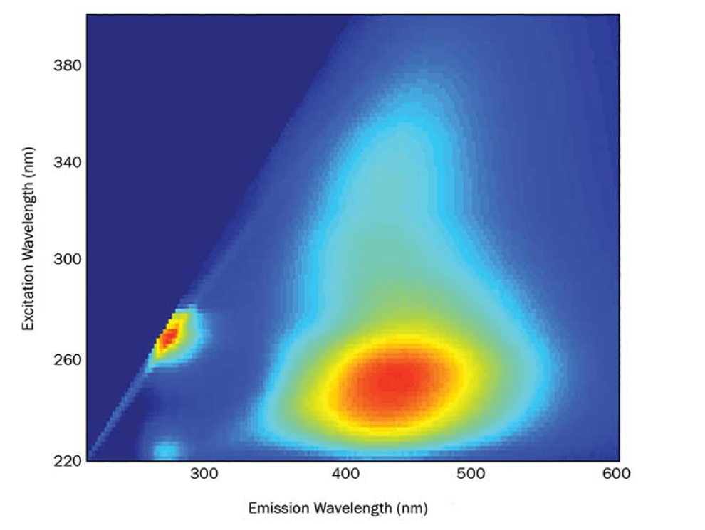
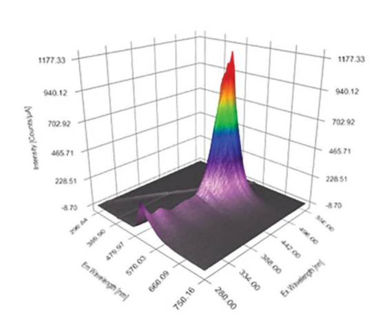
When constructed correctly, an EEM is often referred to as a molecular fingerprint of the sample. The method has proved to be extremely useful in analysing fluorescent molecules in multi-component samples. Examples include the detection and monitoring of chromophoric dissolved organic matter (CDOM) in natural water sources, freshwater ecosystems and similar environmental sample testing. And in food science, EEM methods can assess the quality and origin of foods such as tea, wine and olive oil through an examination of a sample’s unique molecular fluorescence signatures.
Sample Preparation
Careful sample preparation is necessary to achieve a good EEM plot. Perhaps the most important factor is to work with very dilute solutions, if more than a simple qualitative examination is required. All manufacturers recommend diluting the sample, typically to < 0.1 absorbance units. With highly fluorescent compounds, such as sodium fluorescein, working with an even lower absorbance of 0.04-0.08 is perfectly fine. This is to avoid the Inner Filter Effect, which has been described in detail previously.
Measuring sample dilution and absorbance beforehand is recommended, either using a commercial spectrophotometer or some simple and inexpensive absorption spectroscopy setup. The strongest absorption peak in the spectrum should be targeted to be less than 0.1 in absorbance units. If a simple experimental setup is used to do this, remember to record Dark and Reference spectra as well as the Sample, then convert to absorbance units with software.
Rayleigh and Raman Scattering
There will usually be two additional features present when an EEM is recorded. These features present themselves as bands or lines in an EEM. In a sense they are optical artifacts. They are not caused by fluorescence from the sample, but are a result of Rayleigh scattering and Raman scattering. They arise from scattering of the excitation light from the UV light source, primarily by the solvent which is often water. Most spectrofluorometer control software has tools to remove the bands with a few mouse clicks to leave a clean EEM. Both scattering bands are identifiable visually as diagonally-leaning bands from lower left to upper right in an EEM contour map. An example of such bands is shown here for a fluorescent dye sample in deionised water. In this particular example, the Raman band is not visible.
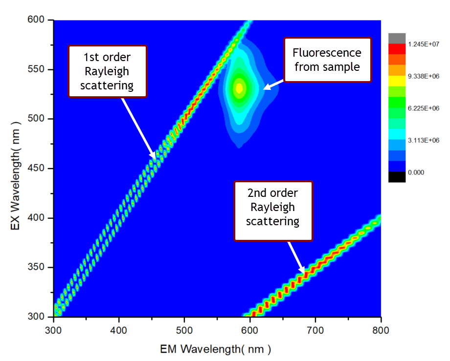
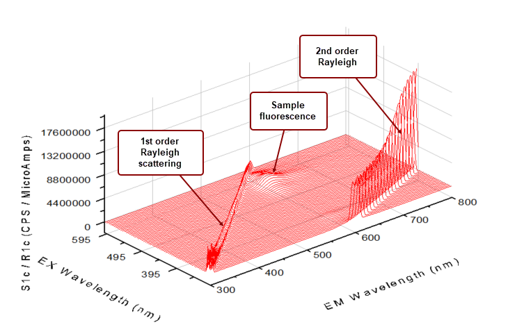
Rayleigh scattering is the elastic scattering of light photons and Raman scattering is an inelastic scattering process. Both mechanisms have been explained in detail in a previous article. Rayleigh scattering occurs without any loss of energy and therefore Rayleigh scattering always appears at the same wavelength as the excitation light. In contrast, Raman scattering is inelastic scattering, where energy is transferred between a scattered photon and the molecule. This results in the scattering band that occurs at a different wavelength to the excitation source.
Water has a relatively weak Raman signal. Whether the band is actually visible in the EEM depends on a number in instrumental factors such as the excitation wavelength and slit width, the integration time, detector sensitivity and fluorescence intensity.
All these features are summarized in the following table:
| Feature | Type | Origin | Relationship |
|---|---|---|---|
|
1st Order Rayleigh |
Elastic Scattering |
Excitation light scattered by sample/solvent |
\(\lambda_{em}=\lambda_{ex}\) |
|
2nd Order Rayleigh |
Elastic Scattering |
Instrument/diffraction-related scattering |
\(\lambda_{em}=2\lambda_{ex}\) |
|
Raman |
Inelastic Scattering |
Molecular vibrations (water/solvent) |
Constant Raman shift in cm\(^{-1}\) |
|
Fluorescence |
Emission |
Excited state relaxation |
Broad emission bands, not scattering lines |
A Two-component Example - Highlighter Pen Fluorescence
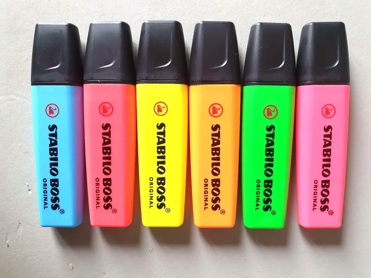
A previous article at Steve’s Open Lab demonstrated how fluorescence spectra of dyes used in highlighter pens can be produced with some basic equipment, such as a UV laser pointer and a small hand-held spectrometer. This simple demo is described in full at this link.
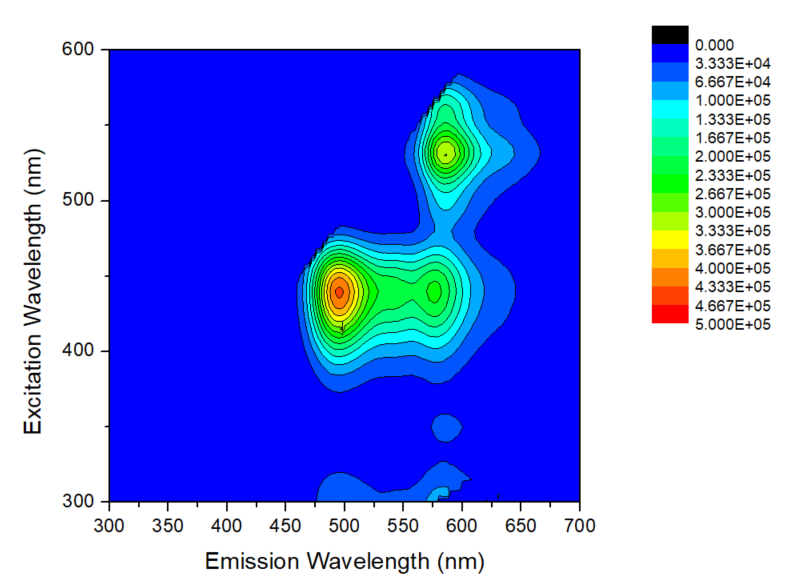
The yellow pen has a strong fluorescence peak in water at about 500 nm from the pyrene-based dye pyranine (Solvent Green 7). The pink pen on the right in the above image contains the dye Rhodamine B with a strong peak at 590 nm. A 1:1 mixture of these two dyes in water serves as a good example to construct a two-component EEM. The “clipping” of the contour lines along one side of the fluorescence peaks is the result of the remocal of the 1st order Rayleigh band by software, as mentioned above (Figure 4).
Final Words...
So that’s the Excitation-Emission Matrix or EEM. Future articles will make use of this molecular fingerprinting technique to analyse multi-component mixtures. Several potential demonstrations already come to mind, such as comparing different cooking oils and monitoring degradation after heating, examining different fruit juices, different types of teas, different natural water sources… the list goes on.
Coming soon to Steve’s Open Lab,