Another Look at Light Emission from Crystals – Part 2
Uncategorized
⏱️ 8 minute read
Introduction
Part 2 of this investigation assumes you have already read Part 1. If not, please stop here and take the 10 minutes or so it will take you to read Part 1 which provides some background to this study and is highly recommended for a full understanding of what follows.
Results with a 2400 Grooves/mm Grating
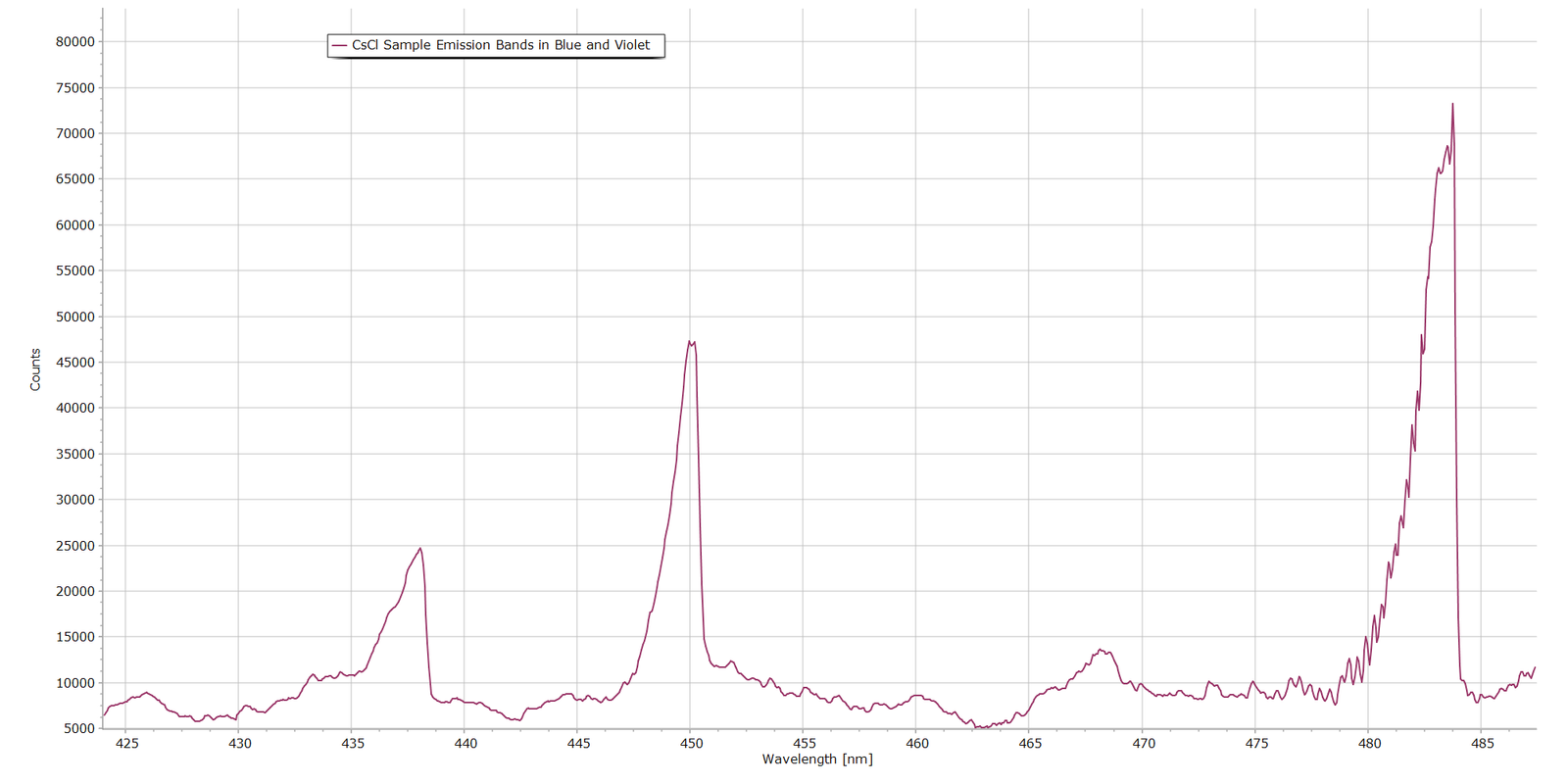
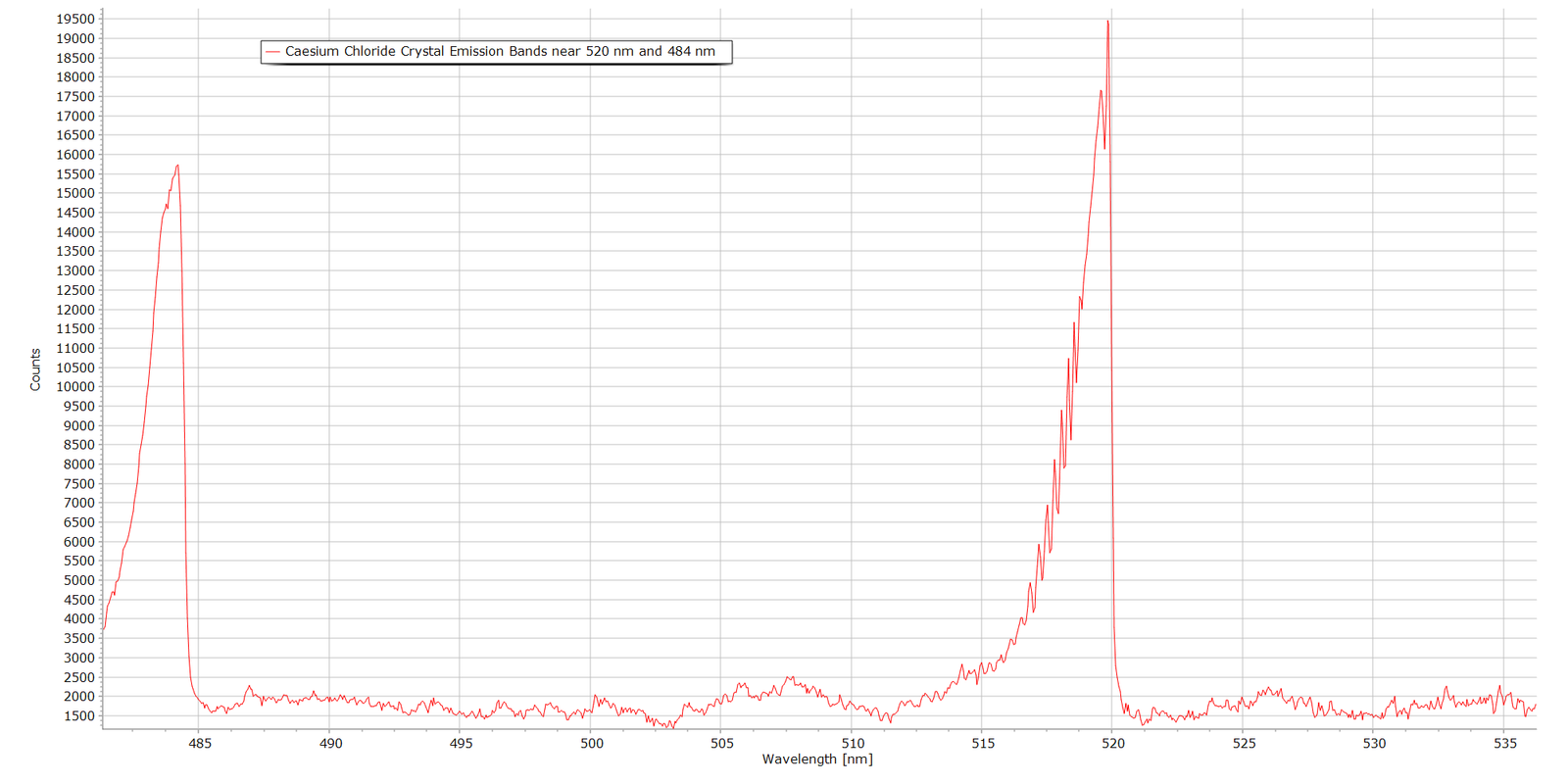
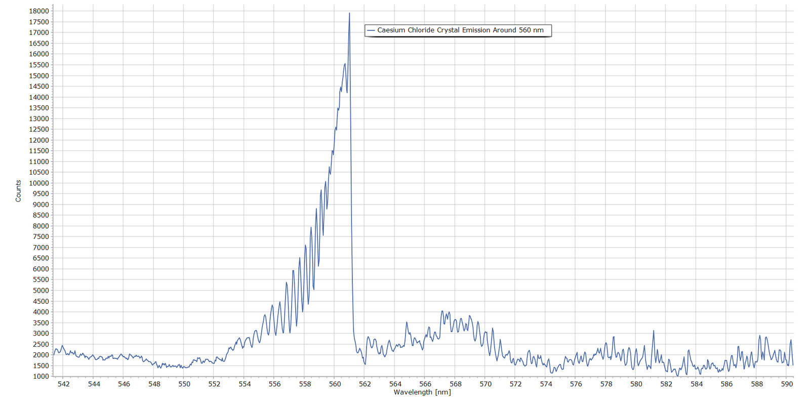
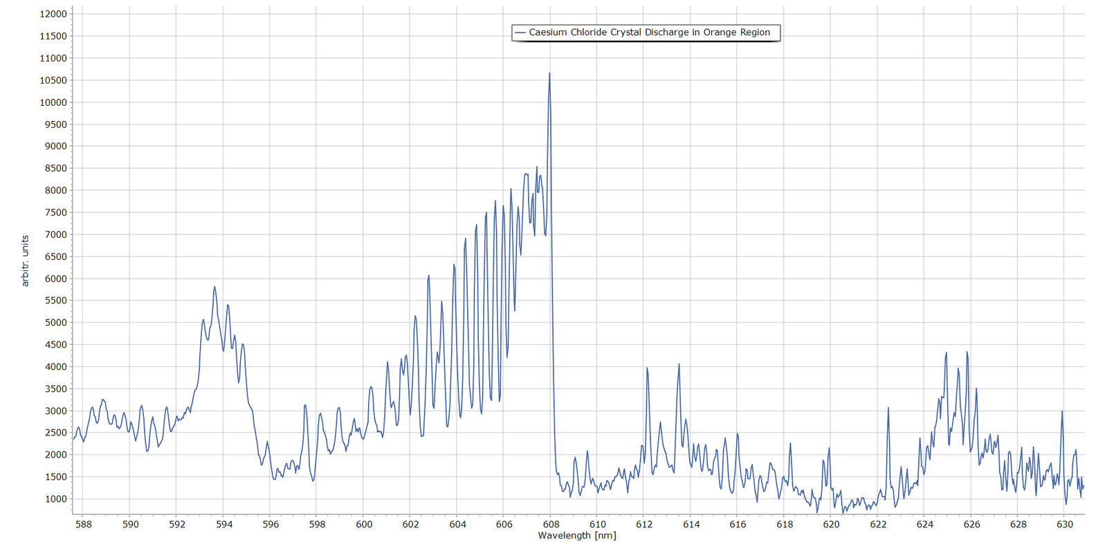
Following on from Part 1, Figures 1 – 5 present spectra of the main emission bands observed in the luminescent glow above the caesium chloride crystals in the discharge. These were obtained with a 2400 grooves/mm diffraction grating and the same MS125 spectrometer with a 25 micron entrance slit.
Fig. 1 The 450nm and 484nm Bands in the CsCl Discharge
Fig. 2 The 464 nm and 520 nm Bands in the CsCl Discharge
Fig. 3 The 560 nm Band in the CsCl Discharge
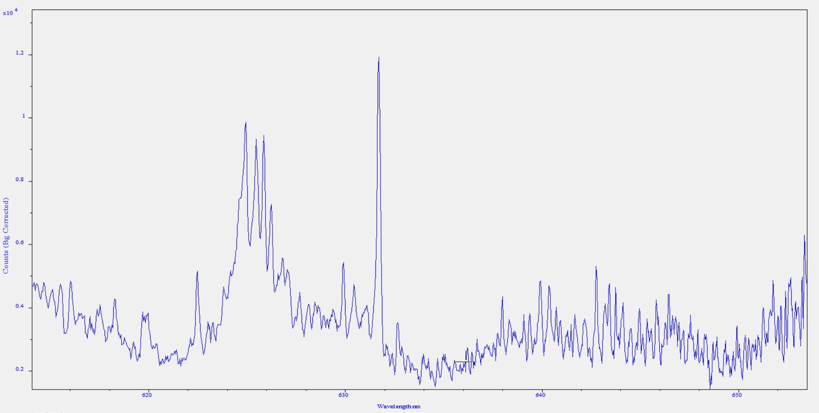
Fig. 4 The 610 nm Band in the CsCl Discharge
Fig. 5 Detail of the Red Region Beyond 610 nm
General Picture
With the possible exception of the spectrum in Fig. 5, what is very clear is that these features are molecular band systems. They are not atomic emission lines. Figs. 2 , 3 and 4 provide the most evidence, where we see well resolved, clear rotational structure on the blue side of each band and a sudden drop in intensity at the position of the band head. In molecular spectroscopy terminology, the bands are “degraded to the blue”. (If the rotational structure had been on the longer wavelength side, the band is described as being degraded to the red.) Fig. 5 is much more complicated, possibly consisting of a mix of molecular and atomic emitters. The chemical nature of these bands still remains to be identified, however. From Part 1 of this article, several potential candidates were proposed, such as Cs*, Cs⁺, Cl, Cl*, Cl₂, Cl₂⁺ and potentially trace impurities from N₂, O₂, H₂O and CO₂.
Analysis and Interpretation Procedure
There are a couple of ways to attempt to distinguish and identify the nature of the chemical species producing these prominent molecular bands:
Option A
Perhaps the more formal approach is to work directly with the raw spectral data and adopt a multi-step procedure such as this:
Take all raw numerical spectral data (wavelengths and intensity values), save in CSV format and import into spreadsheet software.
Convert wavelengths in nanometres to wavenumbers (cm-1), standard practice in spectroscopic analysis.
Calculate absolute values of the separation between adjacent rotational lines, focusing in particular on the convergence of transitions as we approach the different band heads.
Compare differences in λ with standard/official literature measurements and from there make an attempt at identification.
This is quite a lengthy and complex procedure. Furthermore, considering the multi-element nature of possible chemical species emitting in the crystal discharge that were mentioned previously, this is open to error and incorrect spectral assignment.
Option B
A simpler approach, which may be more promising, is to record the spectra of known Cl2 / Cl2+ and CO emitters from other molecules and compare the molecular bands produced by these known emitters with those of the CsCl crystal glow discharge.
Carbon dioxide is an obvious choice here, since in a high voltage electric discharge CO is produced by direct dissociation through these reaction pathways: \[ \mathrm{CO_2 + e^- \rightarrow CO + O + e^-} \] followed by excitation of CO by electron impact, after which excited CO producues Angstrom band emission: \[ \mathrm{CO + e^- \rightarrow CO}(B\,^1\Sigma^+) \mathrm{+ e^-} \]
Other candidate CO emitters are the simple alcohols such as methanol and ethanol. In a discharge, we have
\[ \mathrm{CH_3OH \rightarrow CO + 2H_2} \]
The above equation represents the overall decomposition reaction; the actual discharge chemistry involves several intermediate species, including CH₃, CH₂O, CH, OH and H.
For this analysis, I am adopting the simpler Option B.
The Case for CO
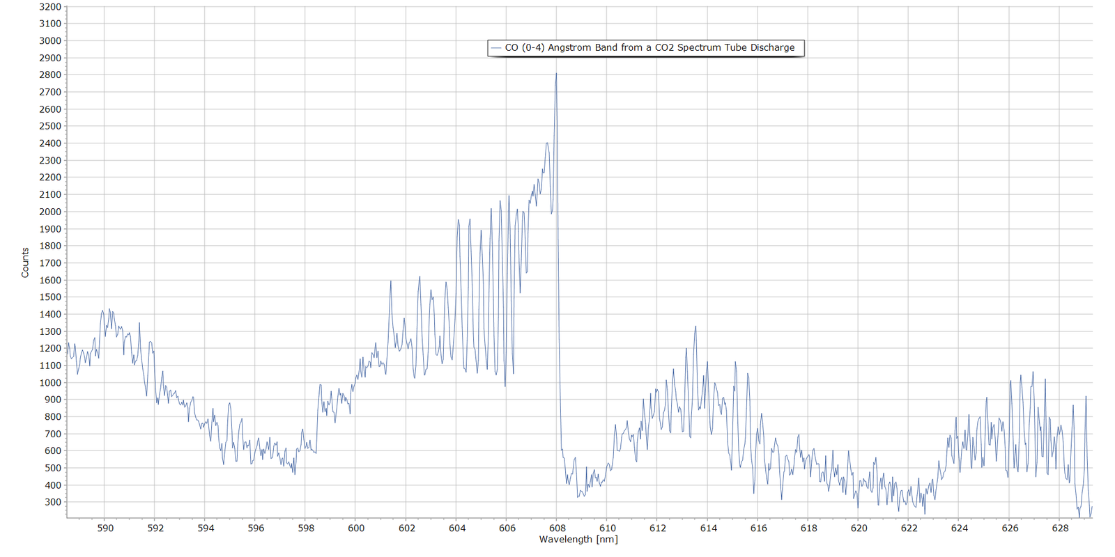
The following spectrum shows emission from carbon dioxide in a discharge. This was produced with a CO2 spectrum tube with exactly the same spectrometer settings used to produce Figs. 1 through 5. This is the CO (0-4) band of the \(B\,^1\Sigma^+ \rightarrow A\,^1\Pi\) electronic transition of carbon monoxide, with vibrational quantum numbers \(v^{\scriptscriptstyle\prime}=0\) and \(v^{\scriptscriptstyle\prime\prime}=4\).
The measured band head here falls at 608.0 nm which is very close to the official NIST reference wavelength of 607.994 nm, compiled by P. Krupenie (Ref. 2).
Fig. 6 The CO (0-4) Angstrom Band Head from a CO2 Spectrum Tube
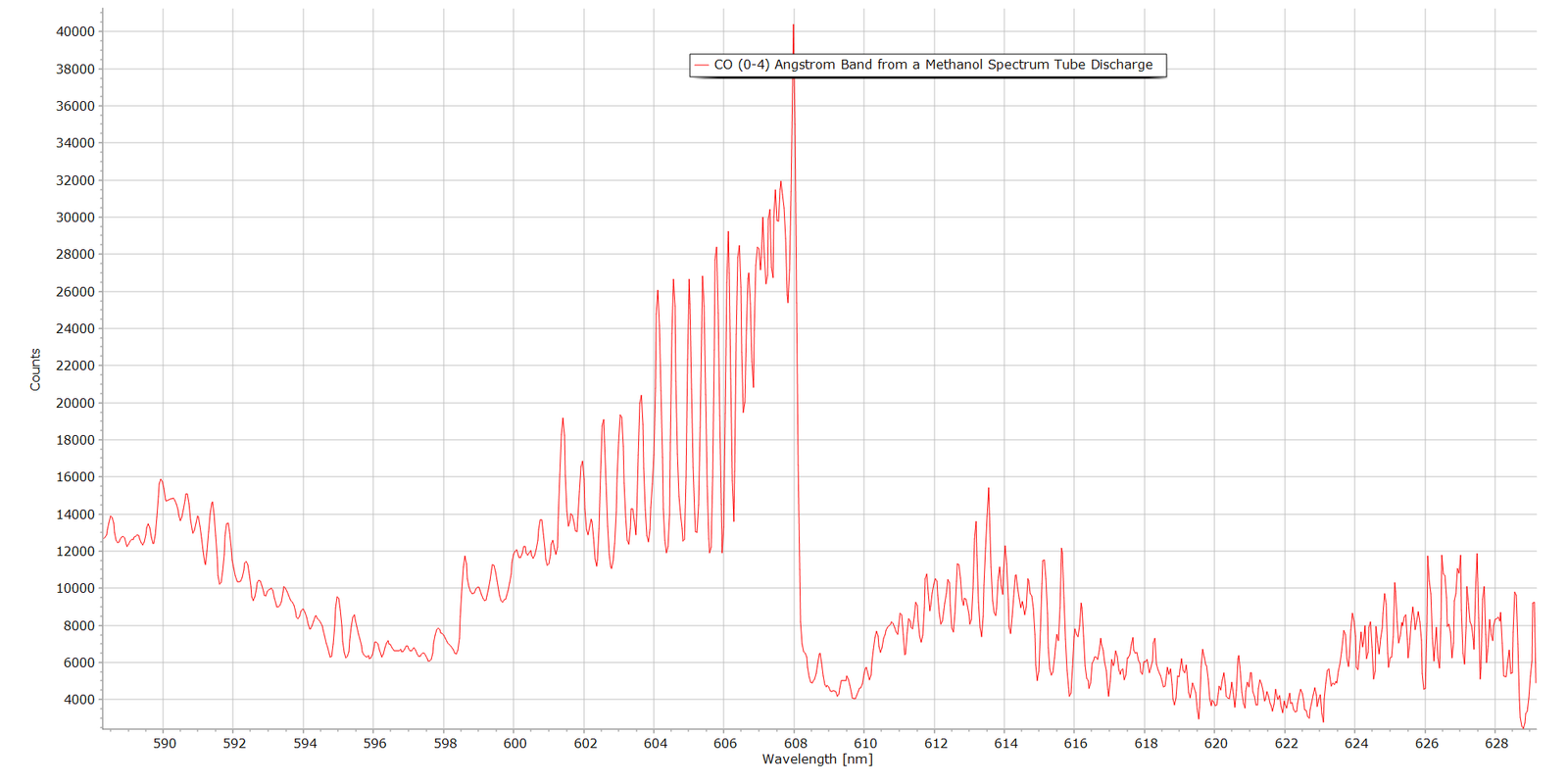
And the following spectrum in Fig. 7 is the same band produced from a methanol vapour spectrum tube. Again, the Angstrom (0-4) band system with associaed rotational structure is very prominent:
Fig. 7 The CO (0-4) Angstrom Band Head Produced from a Methanol Discharge
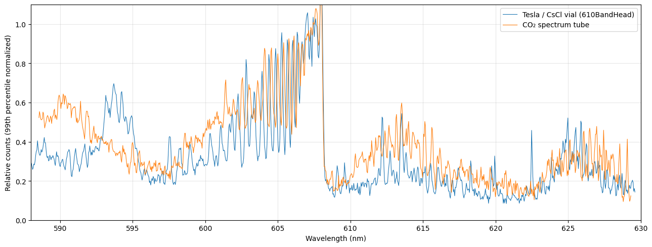
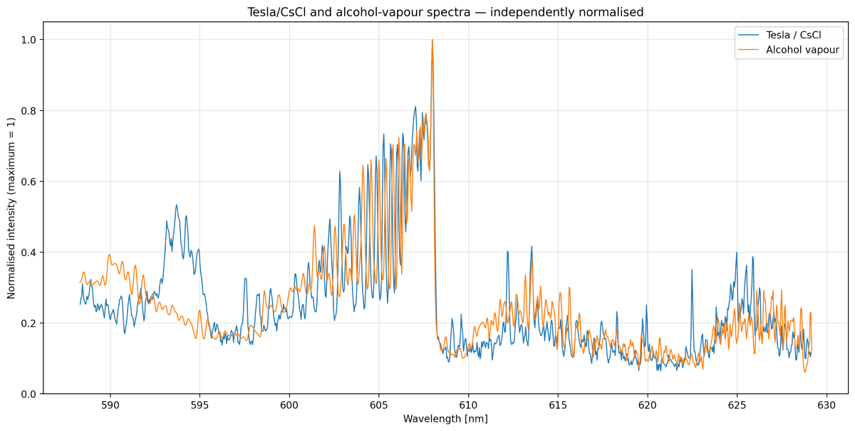
When we superimpose the spectrum from the CsCl discharge in Fig. 4 with either known CO emitter (CO2 or methanol), the wavelength correspondence is remarkably close (Figs. 8 and 9). Note that all superposed/stacked spectra have been normalized for ease of comparison.
Fig. 8 Direct comparison of the 608 nm Band from a CO2 Spectrum Tube and the CsCl Glow Discharge
Fig. 9 Direct comparison of the 608 nm Band from Alcohol Vapour Discharge and the CsCl Glow Discharge
Figs. 8 and 9 superimposed spectra show significant similarity, particularly in the region approximately 600–608 nm where the CO (0-4) molecular band lies, which is of most interest. Although actual line intensities are different, due to different discharge conditions between the CsCl sample vial and the spectrum tube, both exhibit the characteristic progression of closely spaced, increasingly intense molecular band structure, followed by a very abrupt fall in intensity at approximately 608 nm, the band head.
The structured band around 594 nm from the CsCl sample (blue trace) may well be due to other chemical emitters, since it is absent in both the CO₂ and methanol spectra (orange trace).
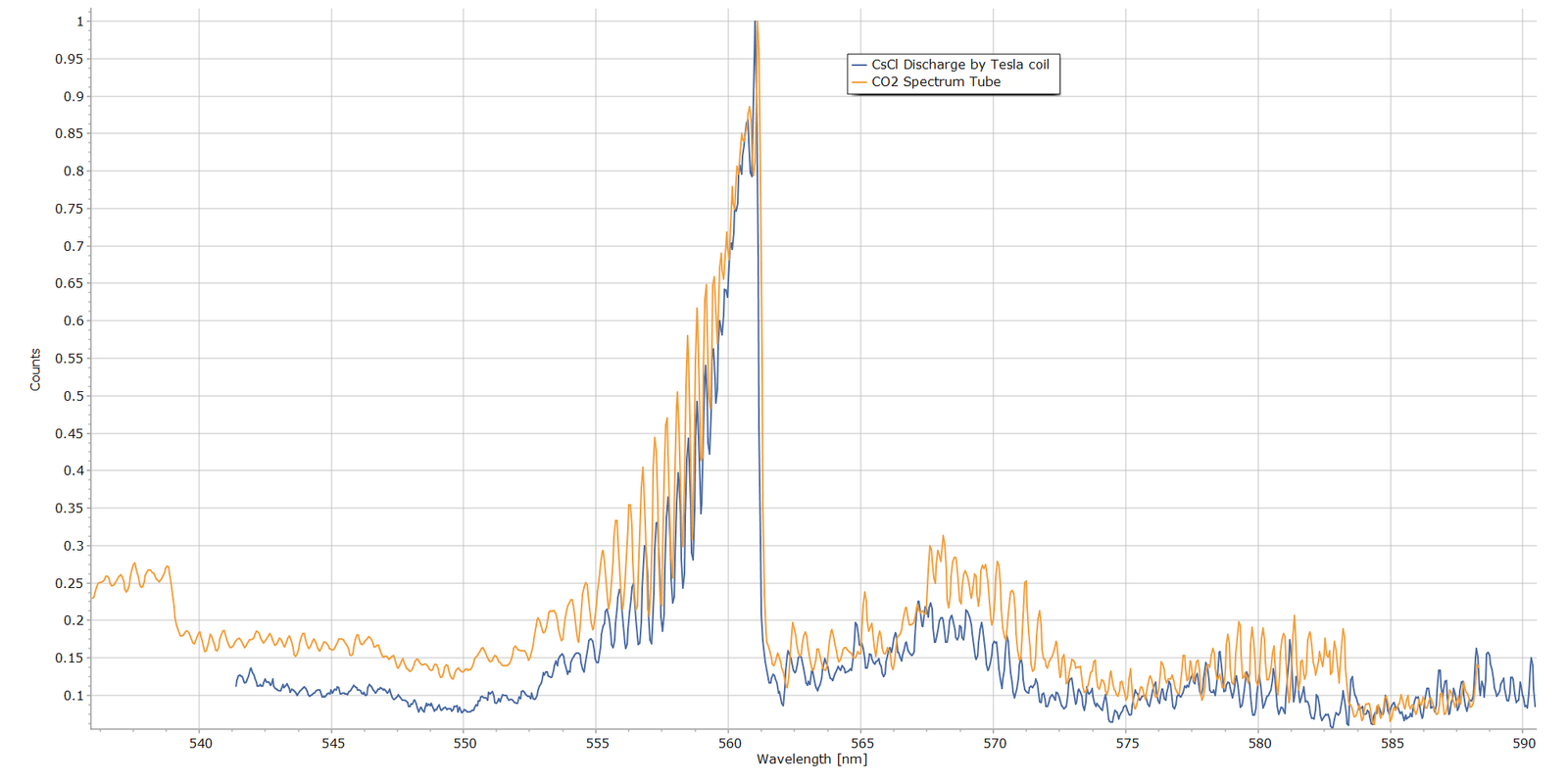
Moving on to the CsCl sample’s molecular band spectrum from Fig. 3, here is the same spectrum stacked with the CO₂ spectrum that exhibits the CO (0-3) Angstrom band:
Fig. 10 Fig. 8 Direct comparison of the 560 nm Band from a CO2 Spectrum Tube and the CsCl Glow Discharge
Again, the wavelength correspondence here is extremely close, providing strong evidence that the caesium chloride emission band is the same as the CO (0-3) Angstrom band of the CO2 discharge.
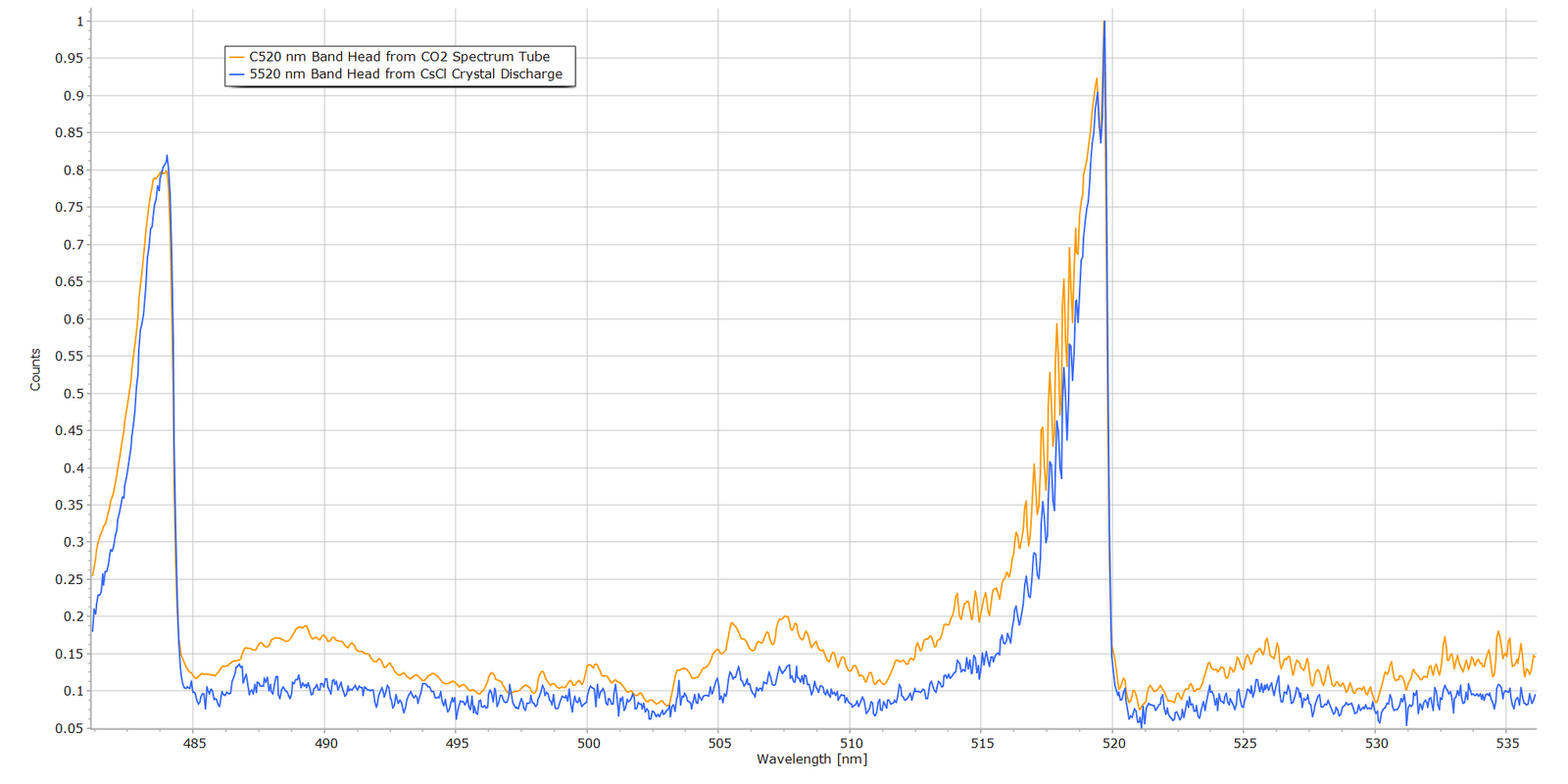
Turning to the CO (0-2) vibronic band at about 520 nm, Fig. 11 displays the band structure from the CO2 discharge and the CsCl discharge:
Fig. 11 Fig. 8 Direct comparison of the 520 nm Band from a CO2 Spectrum Tube and the CsCl Glow Discharge
Wavelength correspondence again is excellent and compelling, particularly the sharp drop in intensity at the band head.
Summary and Conclusions
From the above comparative results, the case for carbon monoxide (CO) as the chemical species emitting in the caesiun chloride crystal glow discharge is extremely strong and compelling. The wavelength positions of the band heads are summarized in the following table and compared to official values from NIST.
Band
NIST (nm) *
CsCl (nm)
CO2 Tube (nm)
(0—0)
451.086
—
449.9469
(0–1)
483.524
—
483.7476
(0–2)
519.822
519.8217
519.8208
(0—3)
561.015
561.0123
561.1015
(0—4)
607.994
607.9848
607.9929
* Official wavelength values taken from NIST/NBS compliation by P. Krupenie, “The Band Spectrum of Carbon Monoxide“, NBS 5, (1966).
It can therefore be concluded, with a high degree of confidence, that the molecular emission bands in the CsCl discharge are the Angstrom bands of carbon dioxide.
As to how C and O atoms form in the discharge is another matter. The most likely explanation is that the CsCl discharge is producing carbon monoxide from trace carbon-containing material inside the vial or from inadequate evacuation of air during manaufacture, since air is 0.04% CO2 by volume. An interesting comment from one reader (thanks Alberto!) is that residues from cleaning solvents, such as iso-propanol, could be present and remain inside the vial prior to sealing. Sample tubes containing solid samples are more difficult to evacuate relative to pure gases, since residual air molecules can become trapped and physisorbed, perhaps even chemisorbed, onto crystal surfaces.
The manufacturer of the CsCl tube samples (Smart-Elements) of the samples was contacted with a request for details of their tube production and air evacuation process. Unfortunately, I am still waiting for a reply, despite several enquiries.
For Technical Enthusiasts...
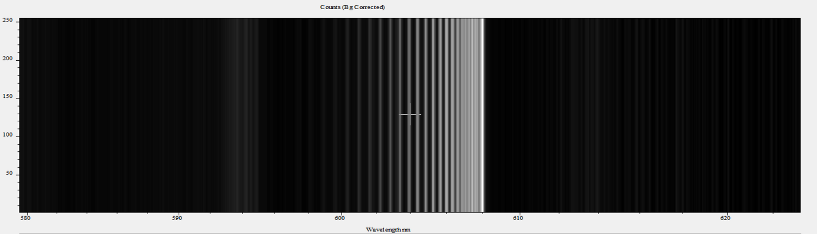
Nothing really to do with the above analysis, but I thought I would add this short information box. Just out of interest, I used the spectrum acquisition software of the spectrometer (Andor Instruments Solis™) to create a synthetic monochrome image of the raw data that created one of the line profiles seen in the above spectra. Here is an example picture of the CO 608 nm band head:
Although created by software, this picture is typical of what atomic and molecular spectroscopists and astronomers had to work with 80+ years ago, using very large laboratory bench spectrographs of up to 5 metres focal length and sometimes even larger. In many instances, molecular bands such as these were much less well defined than the idealized spectrum in Fig. 4. Many examples of these old monochrome spectrograms can be found in G. Herzberg’s classic text Molecular Spectra and Molecular Structure Vol. I, Diatomic Molecules.
The detector of choice in those times was the glass photographic plate, often hypersensitized and “baked” at elevated temperature with forming gas before exposure. This was a non-flammable mixture of 90% nitrogen and 10% hydrogen and was employed to reduce reciprocity failure of the photographic emulsion. Despite hypersensitizing the plates, exposure times could nevertheless extend to minutes or even hours, in order to detect very weak emission lines and bring out vibrational and rotational structure of the molecule under study. In subsequent decades, electronic, and subsequently solid-state, detectors became the mainstay… the photomultipier tubes and charge coupled detectors (CCDs) of today.
References
“Molecular Spectra and Molecular Structure Structure I. Spectra of Diatomic Molecules“, G. Herzberg, 2nd Ed., Van Nostrand, 1950.
“The Band Spectrum of Carbon Monoxide“, Paul H. Krupenie, Institute for Basic Standards, National Bureau of Standards, NBS-5, 1966.
More from the Notebook
Add Your Heading Text Here
From the Laboratory Notebook at Steve's Open Lab
Steve’s Open Lab documents instrument development, independent lab investigations and practical scientific demonstrations. Some articles describe complete experiments, while others record progress in longer-term research projects as new observations become available. Whether you’re looking for a quick experiment or following an ongoing investigation, I hope you’ll find something here that sparks your own curiosity.