
Introduction
Readers of this blog may have noticed that in many of my posts on spectroscopy in the UV and visible, I often use the Newport-Oriel MS125 spectrometer to record spectra. Over the few years since this blog has been running, this little spectrometer has become my go-to workhorse for obtaining UV-visible spectra. Not only for light sources in emission, but also for fluorescence, phosphorescence and occasionally for some reflectance work.
A couple of posts describing this spectrometer were provided previously. The first post introduced the MS125 connected to an older model linear CCD detector, and a second brief article provided an update to the same spectrometer, but with an upgrade to its software in use with a more efficient detector.
In this article, I am going to push the MS125 to its spectroscopic limits, so to speak, in terms of resolution. Spectral resolution is the smallest difference in wavelength (or frequency) that any instrument that disperses light photons is able to distinguish. It is also related to spectral resolving power. The two terms are not exactly the same mathematically, although they are often used interchangeably in technical literature. (You can quickly check online for their exact definitions.)
But before we get started, here’s a quick potted history of the MS125 and its introduction to the R&D community…
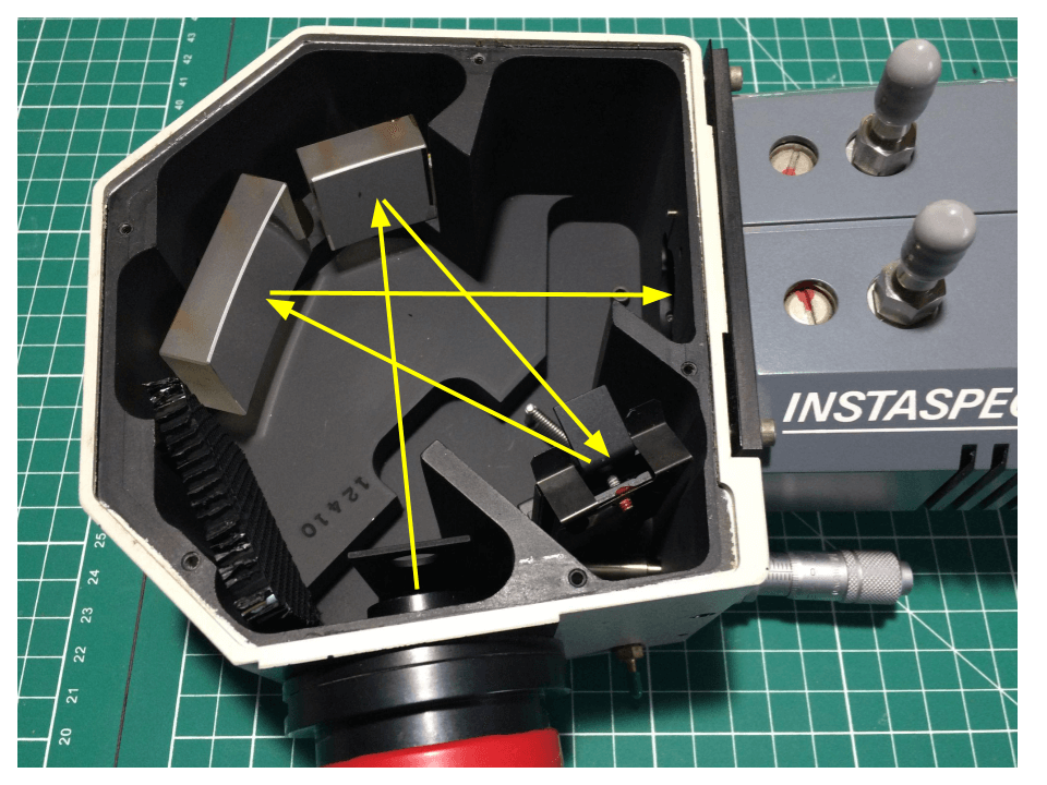
The MS125 spectrometer (or spectrograph) was likely introduced commercially in the very late 1980s or (even more likely) the early 1990s (91-92). The instrument was marketed by Oriel Instruments Inc. as a compact research spectrometer for universities and similar labs. I say “likely introduced” because I did try to determine its first year of manufacture. But after a lot of online searching I have been unable to discover any definite date of initial introduction.
I am lucky to have two of these little spectrometers, whose Oriel catalog model number is 77400. One of them acts as a backup. From the labels on my devices, their manufacturing dates are February 1993 and May 1995. Therefore it is reasonable to assume that the instrument first came into being around the turn of that decade, with perhaps development and testing of prototypes in the late 1980s. If anyone has more exact information, I would be extremely interested in hearing from you via the Comments Panel below ↓
Briefly looking at corporate history and takeovers, the 1990s and 2000s saw a lot of activity, with instrument companies supplying physics and chemistry labs competing intensely for business. Oriel was first acquired by the Thermo Electron company in 1996. Then through a slightly indirect path via Spectra-Physics (a laser manufacturer who at the time were also owned by Thermo Electron), Oriel finished up being owned by Newport Corporation in 2004 when the global behemoth Thermo Electron sold their entire optical technologies businesses to Newport. This is why I sometimes refer to branded equipment on the blog as Oriel-Newport.
But that’s enough history for now. Let’s return to the very purpose of this article: pushing my own MS125 to its practical limits!
Spectral Resolution Testing
Preamble
There are a number of possible atomic emission light sources that can be used practically to test the spectral resolution of any spectrometer.
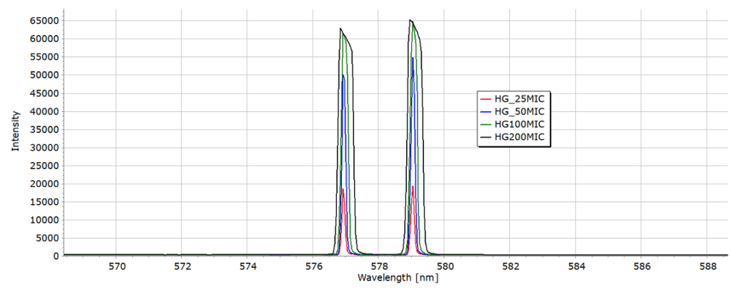
A mercury (Hg) spectral calibration lamp offers an easy test, even for some of the small “hand-held” spectrometers offered by several companies today. Atomic Hg has two fairly weak emission lines at 576.96 and 579.07 nm in the green-yellow region of the spectrum. With a separation of over 2 nm, the large majority of commercial spectrometers on the market (even hand-held ones that increase in performance yearly) should have no trouble in resolving these two lines from atomic mercury (Hg I). Perhaps only with a large entrance slit width and a low pixel-count detector would a spectrometer begin to struggle to resolve these two lines.
A more interesting test could be to try to resolve the Magnesium Triplet in the solar spectrum. This has three Mg lines, this time in absorption, not emission, centred around 517 nm. Or maybe the sodium doublet at 589 nm. Both tests could potentially present a challenge for some spectrometers. For more information on these specific examples, you can link to my articles on the variables affecting spectrometer performance or an evaluation I published a few years ago on one of my DIY spectrometers.
But a far more challenging, even “brutal” test, is to look at the excited atomic oxygen triplet at 777 nm at the extreme edge of the red region in the visible spectrum.
So that is what I am going to attempt with my trusty MS125 in this post – examine this oxygen triplet close up!
Before we start, a quick note on jargon. Often in atomic spectroscopy and in astronomy literature, we see line emission from a neutral atom (using oxygen in this example) referred to as O I, O being the chemical symbol for oxygen. A singly ionised O atom (O+) is then labelled O II, a doubly ionised O atom (O2+) is then labelled O III, and so on. Potentially confusing for the beginner, I admit, but we all get used to it as physics and chemistry students😉.
And why is the 777 nm line actually a triplet in the first place, consisting of three very closely spaced atomic transitions? Well, to answer that (without going into a lot of quantum mechanics), the line is split into three components because of what is termed spin-orbit coupling. This is an interaction of the magnetic moments associated with the spin and orbital motions of the electron. The effect comes under the general name of fine structure splitting. For more information, search online for ‘spin-orbit coupling in atomic spectroscopy’. [However, I would avoid Wikipedia in your search… it goes into far too much detail on relativistic corrections – my personal opinion – which is not required here. Better explanations can be found elsewhere, perhaps starting here.]
The Experiment
Calibrate First!
Before recording any spectra, the spectrometer needs to be properly calibrated in wavelength. And this needs to be done as accurately as possible since we are attempting to split an already narrow atomic emission line into its real three-component triplet observed at high resolution. New calibrations need to be performed each time the grating is rotated to change the wavelength region, or the grating is changed. Therefore great care has to to taken at this stage.
Calibration is performed with good quality ‘pencil-type’ lamps, more details of which are found here. Both neon (Ne) and krypton (Kr) lamps were employed in order to find a sufficient number of emission lines for a good calibration. The resulting raw calibration data are fitted with a 3rd order polynomial expression. Full details on the procedure is described here.
Now the Practical Stuff...
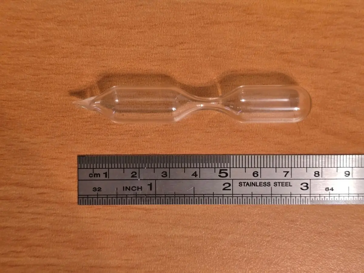
A small sealed glass vial containing pure oxygen at low pressure is used as the sample:
The discharge is generated with a 10-dollar mini Tesla coil widely available online. Light from the glow in the capillary is directed to the entrance slit of the MS125 via a 400 micron optical fibre and an adapter. The adapter has a small internal collimating lens focusing the output light cone that exits the fibre onto the slit. This simple setup is shown here in these three images:
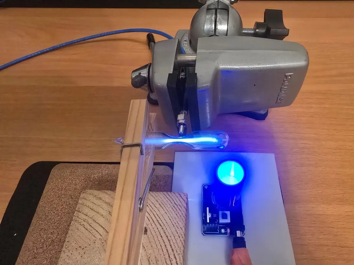
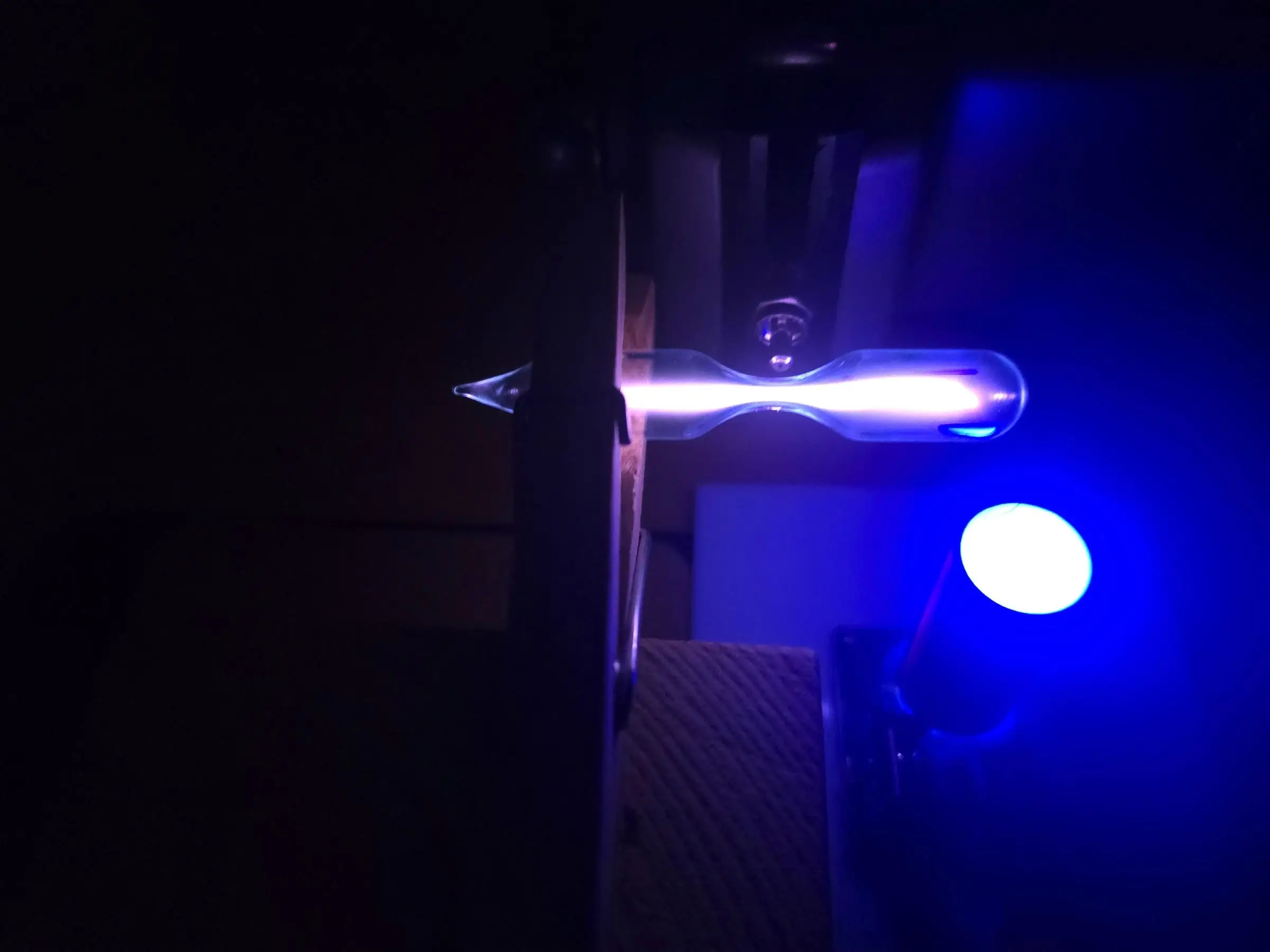
The optical fibre is positioned close to the capillary section of the discharge tube, which is supported with a wooden test-tube holder. The small Tesla is not in contact with the tube, but induces a high frequency, high voltage that ignites and maintains the discharge. The other end of the fibre is attached to the aforementioned adapter, itself clamped to the entrance slit of the MS125.
The Results
With a 600 Groove/mm Grating
With a grating of 600 grooves/mm we obtain a fairly broad survey spectrum of an O2 discharge, extending across much of the visible region and into the near-IR:
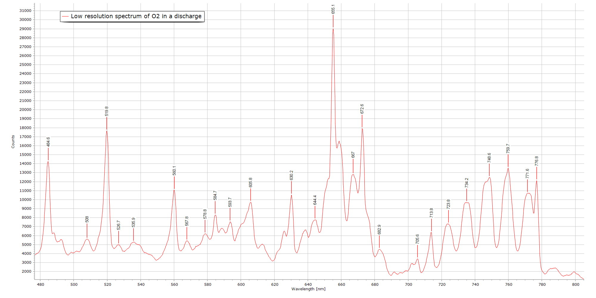
This low-resolution spectrum is a complex mix of O2 molecular bands (many of which overlap) and atomic emission lines. The molecular emission bands arise from electronically excited O₂ and are known to depend strongly on pressure and discharge conditions. What are called the O2 atmospheric bands are visible as well, including emission associated with the O₂(b¹Σg⁺ → X³Σg⁻) electronic transition, notably around 760 nm, as well as other weaker molecular band features. The 760 nm band is often seen in absorption in the solar spectrum, seen here from one of my earlier posts, where I was evaluating a longer focal length home-made spectrometer and a monochrome astronomical CCD camera.
At this resolution the atomic oxygen triplet at 777 nm is totally unresolved and hidden under a much broader structure at this wavelength. In order to attempt to resolve it, we must change the grating and switch to higher resolution.
Result with a 1800 Groove/mm Grating
I skipped over using a 1200 groove grating, anticipating only a modest improvement in spectral resolution there. Fortunately, with an 1800 groove line spacing, covering a wavelength range of about 60 nm, we begin to see some detail of the O I triplet with the MS125…
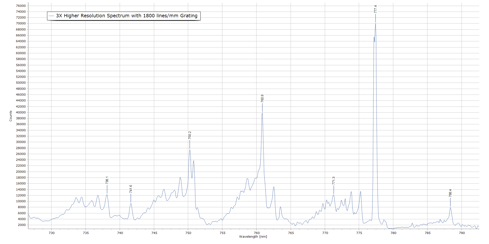
The O I triplet is the intense sharp emission peak at 777 nm in Fig. 2 above, where we can just begin discern a slight “shoulder” on the blue (lower wavelength) edge of this peak. This shoulder becomes much more visible when we zoom in on the region:
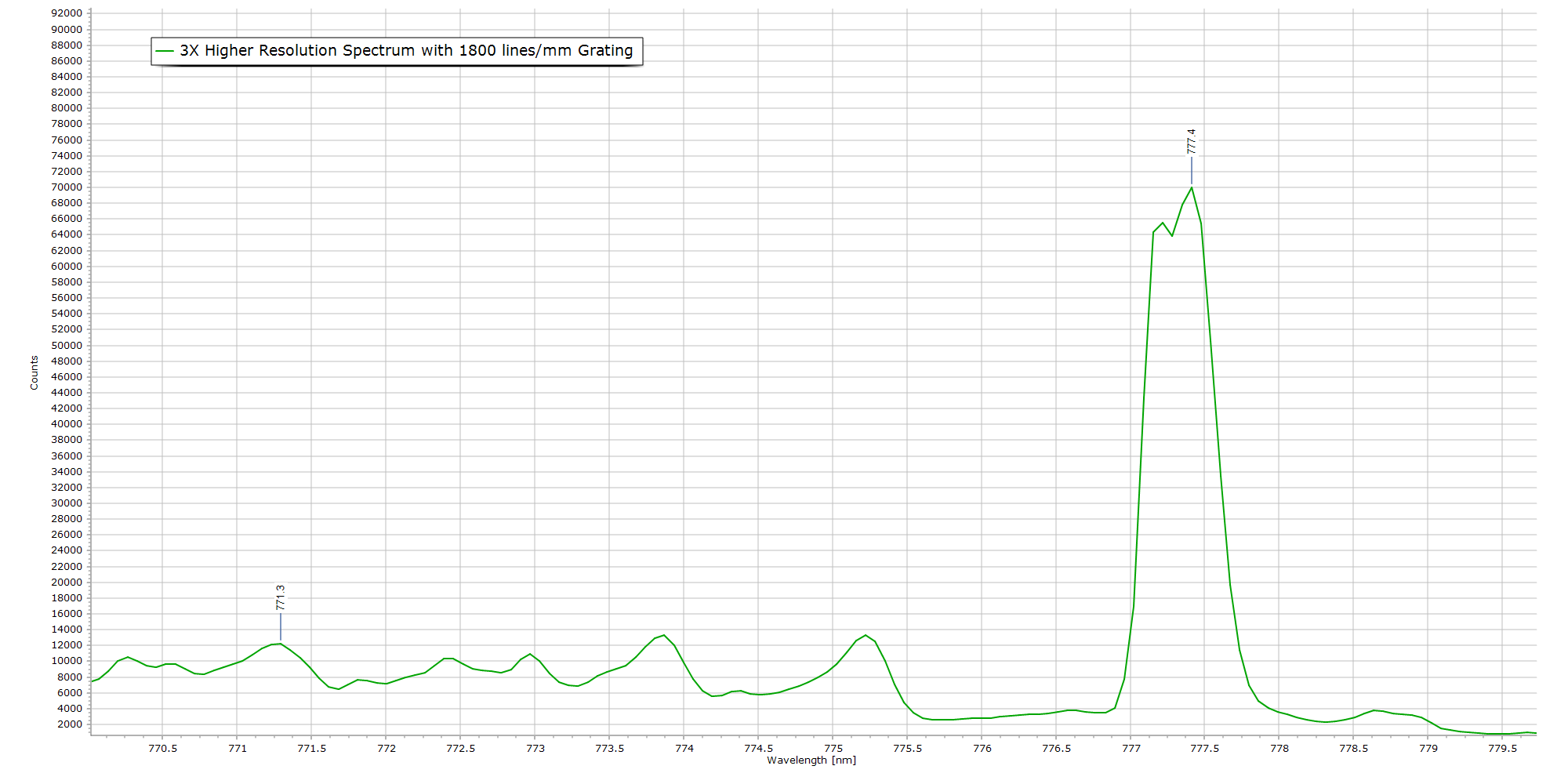
In this zoomed image, major intervals on the wavelength axis are only 0.5 nm (5.0Å) apart! A definite separation of two of the three atomic lines on the blue side of the peak is apparent, and there also appears to be some slight asymmetry on the red edge of this peak, hinting at a third hidden line under the peak profile. (Remember…atomic line transitions are perfectly symmetrical, under ideal conditions, with well aligned and calibrated spectrometers).
How about pushing resolution even more?
At this point, it is decision time. Do I push for even higher spectral resolution with another grating, or do I stop at this point? The answer, in fact, may well be determined by mechanical constraints intrinsic to the MS125, and this is outlined here…
I do have a higher resolution grating for the MS125 with 2400 grooves per mm. And I could very well try it. However, the grating table from my old Oriel user manual, shown below, states that with a 2400 grating, the available spectral range for the MS125 is no further than 625 nm, for a gain in resolution of 0.1 nm (1Å). It is, nevertheless, very tempting to try recording a 2400 spectrum, since an extra 0.1 nm could just be enough to separate the final two components of the oxygen triplet, separated as they are by only 0.122 nm in the above table.
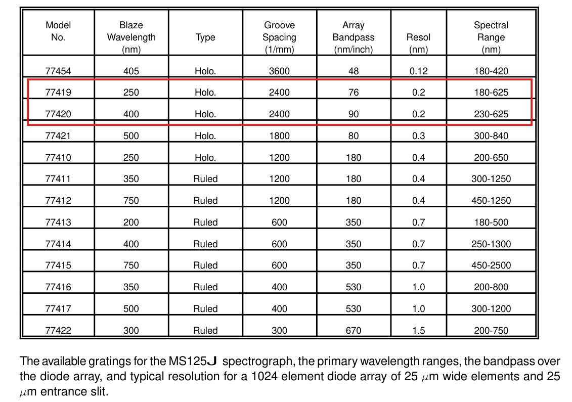
Unfortunately, more recent specs on the exact same spectrometer (see table directly below) have the following information, this time coming from a brief Newport technical brochure.
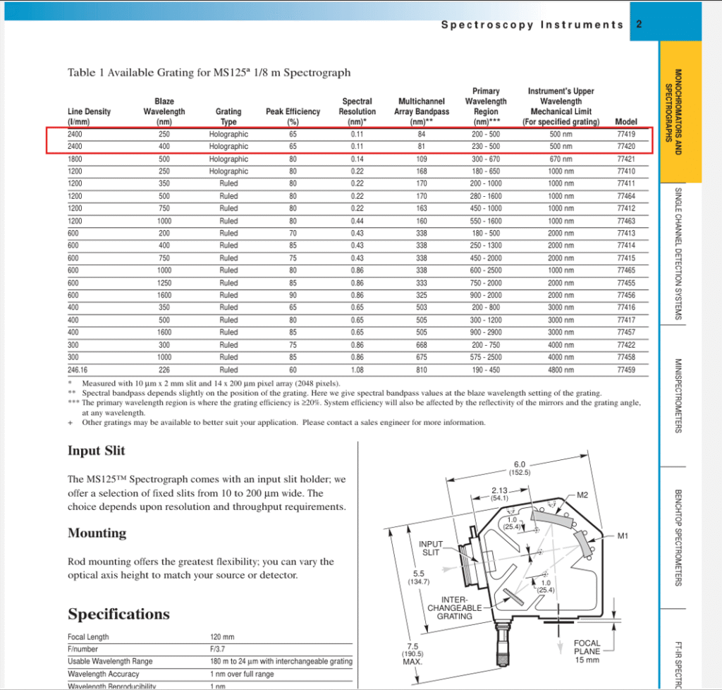
This suggests that the mechanical limit with a 2400 groove per mm grating is only 500 nm and not 625 nm as reported in my original Oriel user manual. This is a huge discrepancy and is likely to be a typo or transcription error from Oriel’s internal documents.
So which is it, Oriel-Newport… a limit of 500 nm or 625 nm? As we shall see now, the whole question may well be moot, as the actual practical issue explains below…
Not the 'Outer Limits', but the Physical Limts
My sincere apologies for the dreadful humour in the title here, but I just couldn’t resist😉. And only readers of a certain age might appreciate it. The problem is as follows:
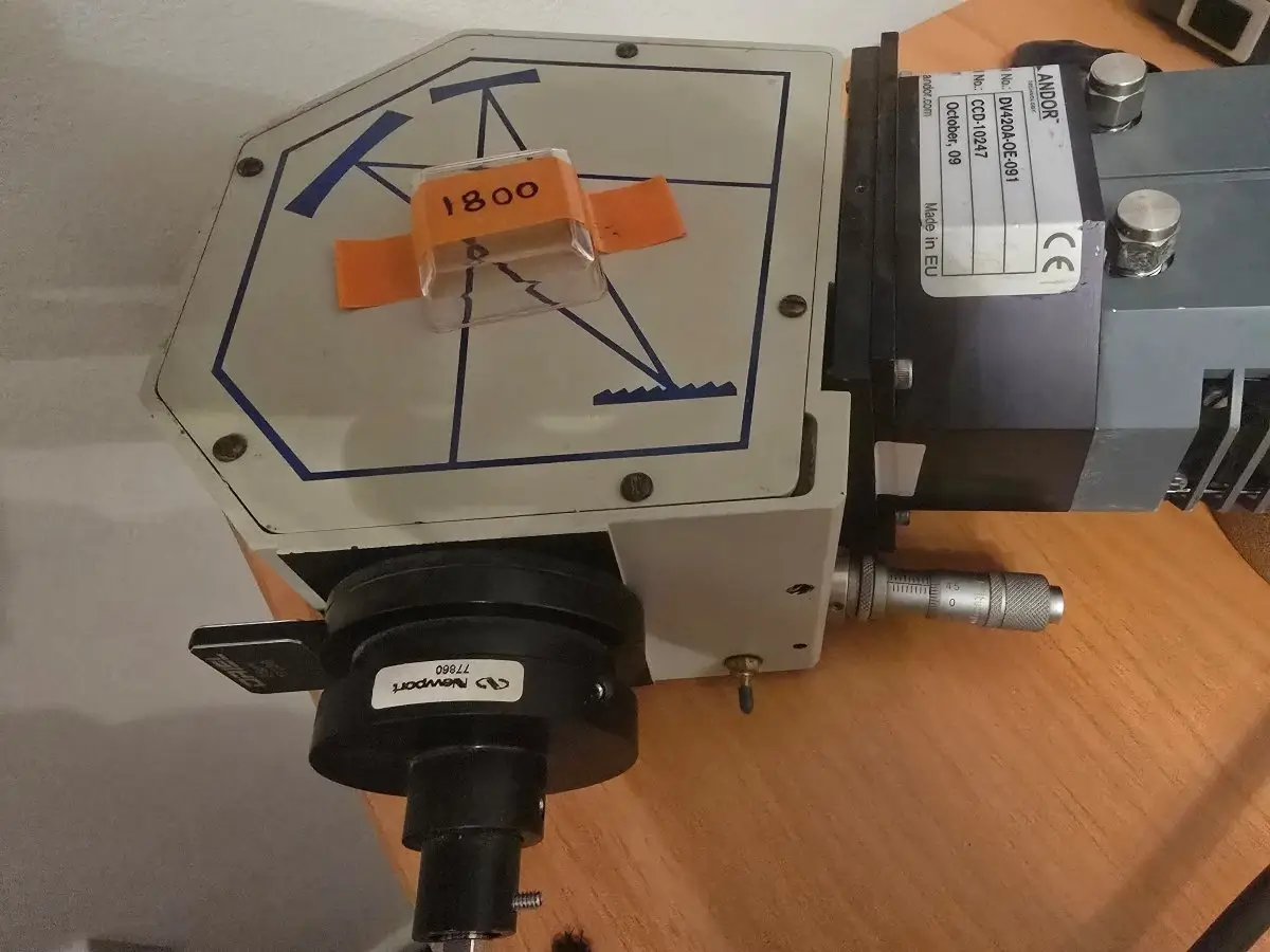
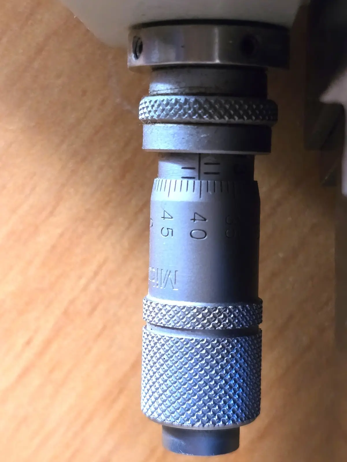
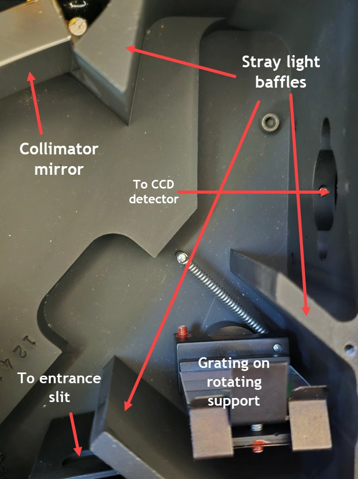
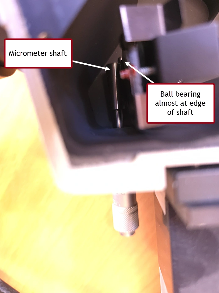
Spectrometers with manually rotatable gratings such as the MS125 use a micrometer screw and a sine-bar drive. These are shown in the closeup pictures just below. (My apologies for the poor depth of field in the third photo.) The sine-bar drive was invented in the early 1980s and described in US Patent 4613233A.
Much more expensive spectrometers employ direct drive designs under computer control. Rotating the grating in this way, either by a sine-bar mechanism or by direct drive, allows different wavelength regions of a spectrum to be studied in detail.
The technical problem with a micrometer sine-bar mechanism is that we always meet an upper wavelength limit mechanically, simply because we always reach the end of the micrometer screw (refer to images). This always happens at the red end of any spectrum because longer (red) wavelengths are dispersed more than shorter (blue) wavelengths with any diffraction grating. Therefore operating at the far red end of the visible spectrum as we are doing will have its limitations, as we rotate the grating angle more and more towards longer wavelengths.
I still do have a little room to play with, since the micrometer vernier scale reading was only 1140 units when I recorded the 1800 groove spectrum. And the vernier scale appears to extend to 1300 units. Whether that small margin is able to achieve a wavelength of 777 nm to become visible to the detector, necessary to observe the oxygen triplet, is not yet known. I could peform the necessary calculations and obtain an estimate, but I am extremely doubtful.
I also want to avoid over-stretching the spring shown in the image. The grating mount is spring-loaded so that the mount always maintains good contact with the micrometer screw via a small ball-bearing. At these micrometer settings the spring is under high tension. However, I do not think this is a problem.
The spring will have been designed by Oriel’s engineers to cope with tensions throughout its full range of micrometer settings. No doubt the hard stop at 1300 is designed to prevent the polished end of the hardened steel micrometer bar losing intimate contact with the bearing! And from the above photo on the right, it appears to be already at the edge of the micrometer shaft. I think I am walking on thin ice here if I push things further!
So for now, I will progress with the analysis of the raw data obtained with the 1800 groove per mm grating. I may return with an attempt at the 2400 groove/mm grating at a later date.
Spectral Resolution Analysis
In order to pursue this analysis we need to work with the raw data, instead of examining the spectral profiles shown in Figs. 2 and 3 earlier. These profiles are simply graphical traces of the data, although we all of us come refer to them as “a spectrum”. They are very useful to appreciate the actual form and shape of any spectrum, since our eyes are far better at identifying very small differences visually; but much less so when we need a thorough numerical analysis.
We also require the most accurate wavelength measurements (in air) on the neutral atomic oxygen triplet (O I) for comparison. The best measurements to date come from NIST (National Institute for Standards and Technology) in the USA. the values are given in Table 1 below, together with line separations and the electronic transitions involved that produce the triplet:
Wavelength (nm) | Wavelength Separation (nm) | Transition | ΔJ |
|---|---|---|---|
777.194 | NA | 3s ⁵S° → 3p ⁵P | -1 |
777.417 | 0.223 | 3s ⁵S° → 3p ⁵P | 0 |
777.539 | 0.122 | 3s ⁵S° → 3p ⁵P | +1 |
Table 1. Official NIST Data for the O I Triplet Emission Lines of Neutral Atomic Oxygen
I exported the data into a spreadsheet app as a CSV file. This gives us two long columns of numbers, corresponding to Counts (Y axis) and Wavelength (X axis), plus their header labels. There are 1024 of each – the number of pixels on the CCD sensor. Focusing our attention to the O I triplet at 777 nm, here are the wavelength values measured by the MS125 with corresponding intensities (counts) detected by the CCD:
Wavelength (nm) | Counts | Comments |
|---|---|---|
777.0905 | 43495 | |
777.1549 | 64345 | |
777.2193 | 65511 | ← first resolved maximum |
777.2837 | 63813 | |
777.3841 | 67787 | |
777.4125 | 70041 | ← second resolved maximum |
777.4769 | 65487 | |
777.5413 | 50589 | ← third line expected here |
777.6057 | 33475 | |
777.6702 | 19654 |
The good news is that the O I triplet is being partially resolved 😎. The two strongest local maxima have differences of only +0.03 nm and -0.01 nm relative to official NIST values:
Measured Line (nm) | NIST Ref. Wavelength (nm) | Difference |
|---|---|---|
777.219 | 777.194 | +0.03 nm |
777.413 | 777.420 | -0.01 nm |
The expected third emission line is at 777.54 nm. The data do not show it as a distinct third maximum, but the profile extends asymmetrically through this region. This can be seen by referring to the zoomed spectrum in Fig. 3, where there is a slight asymmetry, with the red side of the peak tailing off more slowly than the blue side.
Numerical Modelling Approach
In order to take the analysis further, the approach I use is to consider the 777 nm peak as three overlapping line profiles (effectively instrumental line profiles) and to constrain their wavelength separations to the officially known NIST O I triplet separations.
This means that the optimizing process, which essentially applies the non-linear least squares method, cannot independently move the three oxygen lines around to obtain a better fit. It can shift the entire triplet left or right, but the lines’ separations remain fixed at the official NIST separations of 0.223 nm and 0.122 nm. This is probably a better approach than allowing an iterative optimization routine to obtain a fit simply by moving around three completely free Gaussian curves.
A common offset can be used, and a common Gaussian line width, but with three independent amplitudes, which are the emission line intensities in units of counts.
From the fit, it should then be possible to estimate the actual FWHM (Full Width at Half Maximum) at 777 nm and from that, to determine quantitatively whether or not there does exist a third O I line present at the red end of this feature.
That’s the overall strategy. It is not possible to perform this level of modelling in standard spreadsheet software. The best approach I was able to find online was within the Python programming landscape, with the aide of several subroutines and Python libraries.
The CSV data were first imported into Pandas. This is a Python library used for handling large data sets. SciPy was used for the non-linear least-squares fitting procedure (specifically the command scipy.optimize.least_squares). NumPy performed all the necessary numerical calculations and Matplotlib generated the fitted plot. The resulting plot can be seen here:
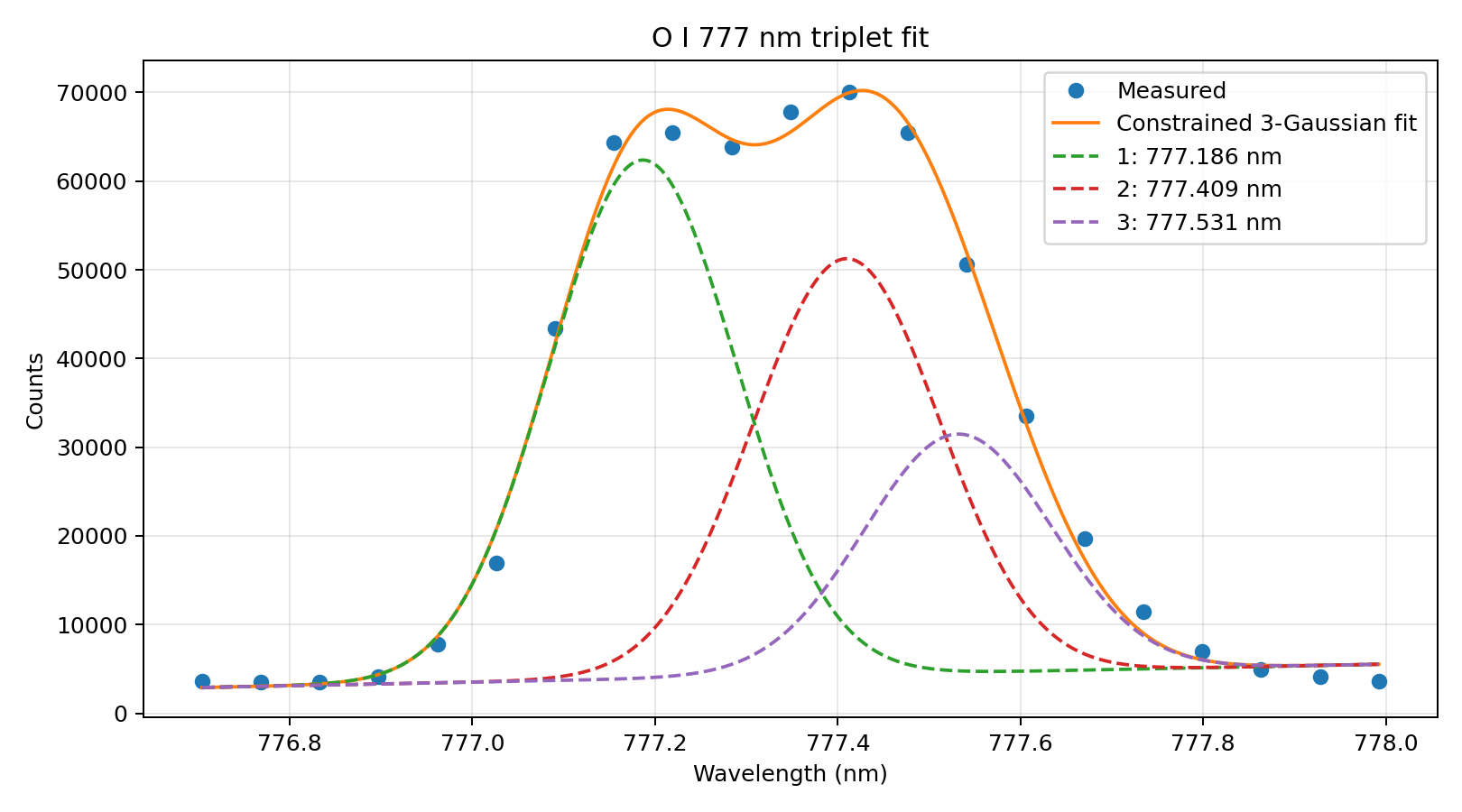
The constrained 3-Gaussian fit appears to have worked very well. Blue dots in the plot are the actual data points measured by the spectrometer. The orange line is the 3-Gaussian fit to this data, and the three individual Gaussians are represented by the three dotted curves, whose peak maxima are 777.1863, 777.4093 and 777.5313 nm from left to right. These values are in very good agreement with the official NIST wavelength values for the oxygen triplet.
ID | Fitted Value (nm) | NIST Wavelength (nm) | Difference |
|---|---|---|---|
Gaussian 1 | 777.1863 | 777.1944 | 0.0081 |
Gaussian 2 | 777.4093 | 777.4166 | 0.0073 |
Gaussian 3 | 777.5313 | 777.5388 | 0.0075 |
The fitted values correspond to an average offset of only 0.0077 nm from NIST measurements. The common fitted Gaussian FWHM is 0.241 nm, which implies an effective resolving power R of the MS125 spectrometer at this wavelength of ≈ 3230. Model fit quality is high, with R² = 0.9961 and an RMS residual of about 1664 counts.
When it comes to the strengths of the three emission lines, relative intensities of the modelled peaks do not perform too badly either. Relative intensity values from NIST report values of 870, 810 and 750 for the three lines (lowest wavelength first). This corresponds to line ratios of 1.00 : 0.93 : 0.86. Fitted relative amplitude ratios from the model are about 1.00 : 0.80 : 0.46.
The difference is readily explained by the different conditions in the discharge. The intensities of all gaseous elements excited in low pressure gas discharges are sensitively dependent on conditions. The pressure in the tube, the applied voltage used to strike and then maintain the plasma, tube geometry and electron densities can all affect the intensities of spectral lines observed in a spectrometer. Even the values in the NIST data are transcribed from literature papers that may well be using different discharge conditions. Therefore it is no surprise that the modelled relative intensities are somewhat different from NIST ratios.
What is far more important is the excellent agreement and correspondence in wavelengths between NIST values and the measured and modelled data.
This is remarkable for a spectrometer of this size!
Conclusions
The MS125 has shown itself to be an excellent little spectrometer!
With an 1800 grooves/mm grating and a 25 μm entrance slit, the MS125 partially resolves the neutral oxygen 777 nm triplet, always a challenge for many spectrometers. That is a feat in itself!
In addition, a constrained three-component Gaussian fit reproduces the observed triplet line profile extremely well, indicating that all three members of this multiplet contribute to the measured emission band at 777 nm.
It is clear that the instrument is capable of considerably more than its modest size would suggest. Although named the MS125, implying a focal length of 125 mm, the actual focal length is closer to 120 mm from its technical specifications. So this result is all the more surprising and pleasing.
This performance may well be helped by the MS125’s high build quality. The walls and optical bench, including well-designed stray light baffles, are machined from one single block of aluminium. Only the lid of the spectrometer is a separate item, to allow access for changing the grating. The two reflective optics employed for collimating and focusing, are thick, solid looking good quality mirrors locked and sealed firmly in place on their mounts.
With its high degree of flexibility for changing slit widths and diffraction gratings, it is no surprise that this little spectrometer has been very popular with R&D labs for well over 40 years.
Thanks for your patience with this longer than usual post, and for getting to the end. 😊
1 thought on “Pushing the Limits of a Small Spectrometer”
Dear Steve,
Great post, and a great introduction to the NIR emission spectroscopy of spectrum tubes, a largely unexplored area for the amateur. With my night vision scope, visible-blocking/NIR- transmitting filter, and cheap “rainbow glasses”, I can see the two atomic oxygen lines at 777 & 845 nm, but only as single bright lines. Fantastic job splitting the brighter line at 777 nm into the triplet we have all heard about but never seen!
Respectfully,
Gerry Francisco